.ipynb .pdf

repository open issue suggest edit

Binder

Contents

Geospatial Transforms

Instructors: Tyler Sutterley, Hannah Besso and Scott Henderson, some material adapted from David Shean

Learning Objectives

• Review fundamental concepts of geospatial coordinate reference systems (CRS)

• Learn how to access CRS metadata

• Learn basic coordinate transformations relevant to ICESat-2

Introduction

ICESat-2 elevations are spatial point data. Spatial data contains information about where on the surface of the Earth a certain feature is located, and there are many different ways to define this location. While this seems straightforward, two main characteristics of the Earth make defining locations difficult:

1. Earth is 3-dimensional (working with spatial data would be a lot easier if the world were flat)!

2. Paper maps and computer screens are flat, which causes issues when we try to use them to display rounded shapes (like the Earth’s surface). Making things even more difficult, the irregular shape of the Earth means there is no one perfect model of its surface on which we could place our spatial data points! Instead, we’re left with many models of the Earth’s surface that are optimized for different locations and purposes.

import geopandas as gpd
import hvplot.xarray
from IPython.display import Image
import matplotlib.patches
import matplotlib.pyplot as plt
from mpl_toolkits import mplot3d
import netCDF4
import netrc
import numpy as np
import os
import osgeo.gdal, osgeo.osr
import pyproj
import rasterio
import rasterio.features
import rasterio.warp
import rioxarray
import re
import warnings
import xarray as xr
# import routines for this notebook
import utilities
# turn off warnings
warnings.filterwarnings('ignore')

%matplotlib inline
%config InlineBackend.figure_format = 'retina'

Let’s Start by Making a Map 🌍

Q: Why would we use maps to display geographic data?

Geopandas vector data

We’ll use geopandas built-in Natural Earth dataset to load polygons of world countries

# Load a dataset consisting of land polygons
world = gpd.read_file(gpd.datasets.get_path('naturalearth_lowres'))
world.head()

	pop_est	continent	name	iso_a3	gdp_md_est	geometry
0	920938	Oceania	Fiji	FJI	8374.0	MULTIPOLYGON (((180.00000 -16.06713, 180.00000...
1	53950935	Africa	Tanzania	TZA	150600.0	POLYGON ((33.90371 -0.95000, 34.07262 -1.05982...
2	603253	Africa	W. Sahara	ESH	906.5	POLYGON ((-8.66559 27.65643, -8.66512 27.58948...
3	35623680	North America	Canada	CAN	1674000.0	MULTIPOLYGON (((-122.84000 49.00000, -122.9742...
4	326625791	North America	United States of America	USA	18560000.0	MULTIPOLYGON (((-122.84000 49.00000, -120.0000...

This 👇 will create a map with global coastlines

fig,ax1 = plt.subplots(num=1, figsize=(10,4.55))
minlon,maxlon,minlat,maxlat = (-180,180,-90,90)

world.plot(ax=ax1, color='0.8', edgecolor='none')

# set x and y limits
ax1.set_xlim(minlon,maxlon)
ax1.set_ylim(minlat,maxlat)
ax1.set_aspect('equal', adjustable='box')

# add x and y labels
ax1.set_xlabel('Longitude')
ax1.set_ylabel('Latitude')

# adjust subplot positioning and show
fig.subplots_adjust(left=0.06,right=0.98,bottom=0.08,top=0.98)

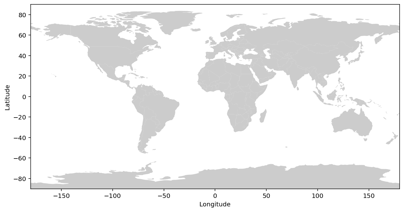
Q: So how did we just display a rounded shape on a flat surface?

Geographic Coordinate Systems

Locations on Earth are usually specified in a geographic coordinate system consisting of

• Longitude specifies the angle east and west from the Prime Meridian (102 meters east of the Royal Observatory at Greenwich)

• Latitude specifies the angle north and south from the Equator

The map above projects geographic data from the Earth’s 3-dimensional geometry on to a flat surface. The three common types of projections are cylindric, conic and planar. Each type is a different way of flattening the Earth’s geometry into 2-dimensional space.

Cylindric	Conic	Planar

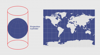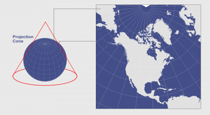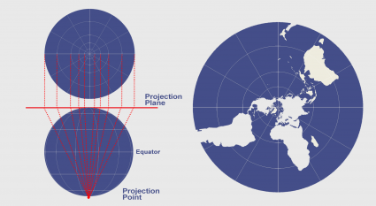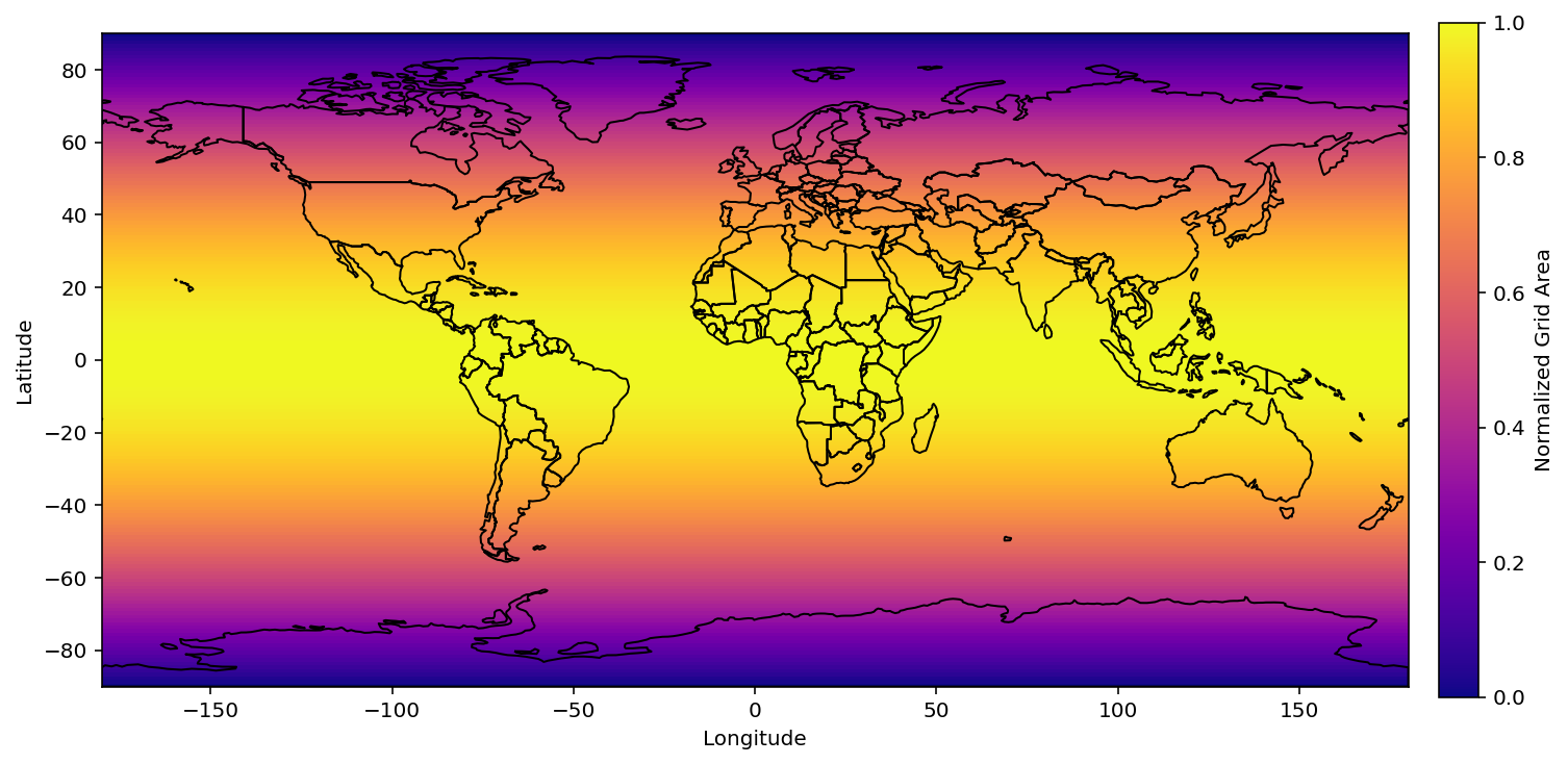
This map is in an Equirectangular Projection (Plate Carrée), where latitude and longitude are equally spaced. Equirectangular is cylindrical projection, which has benefits as latitudes and longitudes form straight lines.

Warning

While simple conceptually, this projection distorts both shape and distance, particularly at higher latitudes! So it is not a great choice for data analysis.

To illustrate distortion on this map below 👇, we’ve colored the normalized grid area at different latitudes below:

fig,ax1 = plt.subplots(num=1, figsize=(10.375,5.0))
minlon,maxlon,minlat,maxlat = (-180,180,-90,90)
dlon,dlat = (1.0,1.0)
longitude = np.arange(minlon,maxlon+dlon,dlon)
latitude = np.arange(minlat,maxlat+dlat,dlat)

# calculate and plot grid area
gridlon,gridlat = np.meshgrid(longitude, latitude)
im = ax1.imshow(np.cos(gridlat*np.pi/180.0),
    extent=(minlon,maxlon,minlat,maxlat), 
    interpolation='nearest',
    cmap=plt.cm.get_cmap('plasma'),
    origin='lower')

# add coastlines
world = gpd.read_file(gpd.datasets.get_path('naturalearth_lowres'))
world.plot(ax=ax1, color='none', edgecolor='black')

# set x and y limits
ax1.set_xlim(minlon,maxlon)
ax1.set_ylim(minlat,maxlat)
ax1.set_aspect('equal', adjustable='box')

# add x and y labels
ax1.set_xlabel('Longitude')
ax1.set_ylabel('Latitude')

# add colorbar
cbar = plt.colorbar(im, cax=fig.add_axes([0.92, 0.08, 0.025, 0.90]))
cbar.ax.set_ylabel('Normalized Grid Area')
cbar.solids.set_rasterized(True)

# adjust subplot and show
fig.subplots_adjust(left=0.06,right=0.9,bottom=0.08,top=0.98)

The Components of a Coordinate Reference System (CRS):

• Projection Information: the mathematical equation used to flatten objects that are on a round surface (e.g. the earth) so you can view them on a flat surface (e.g. your computer screens or a paper map).

• Coordinate System: the X, Y, and Z grid upon which your data is overlaid and how you define where a point is located in space.

• Horizontal and vertical units: The units used to define the grid along the x, y (and z) axis.

• Datum: A modeled version of the shape of the earth which defines the origin used to place the coordinate system in space.

👆 Borrowed from Earth Data Science Coursework

Notes on Projections

• There is no perfect projection for all purposes

• Not all maps are good for ocean or land navigation

• Not all projections are good for polar mapping

• Every projection will distort either shape, area, distance or direction:

  • conformal projections minimize distortion in shape

  • equal-area projections minimize distortion in area

  • equidistant projections minimize distortion in distance

  • true-direction projections minimize distortion in direction

While there are projections that are better suited for specific purposes, choosing a map projection is a bit of an art 🦋

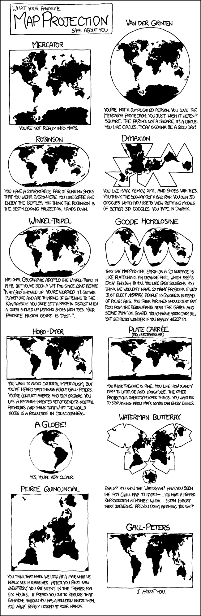
👆 Obligatory xkcd

Q: What is your favorite projection? 🌎

Q: What projections do you use in your research? 🌏

Determine your data’s CRS

Using geopandas, we can get CRS information about our data:

world.crs

<Geographic 2D CRS: EPSG:4326>
Name: WGS 84
Axis Info [ellipsoidal]:
- Lat[north]: Geodetic latitude (degree)
- Lon[east]: Geodetic longitude (degree)
Area of Use:
- name: World.
- bounds: (-180.0, -90.0, 180.0, 90.0)
Datum: World Geodetic System 1984 ensemble
- Ellipsoid: WGS 84
- Prime Meridian: Greenwich

EPSG: European Petroleum Survey Group. Back in the day, this group created codes to standardize how different reference systems were referred to, and now EPSG codes are widely used in geospatial work! There are several websites that let you navigate the entire EPSG database: https://epsg.io/4326

If CRS metadata on any products isn’t included within the data product, make sure it’s in the right projection and datum. Often metadata reports or readme files will provide this information.

Reproject your data

And we can also reproject it fairly easily, as long as our vertical reference (our ellipsoid or geoid) stays the same. For example, let’s use epsg:3031, which uses the same Datum, but is otherwise very different.

• Remember: “The projection is the mathematical equation used to flatten objects that are on a round surface (e.g. the earth) so you can view them on a flat surface (e.g. your computer screens or a paper map).”

world_antarctic = world.to_crs('epsg:3031')

Did it work?

world_antarctic.crs

<Derived Projected CRS: EPSG:3031>
Name: WGS 84 / Antarctic Polar Stereographic
Axis Info [cartesian]:
- E[north]: Easting (metre)
- N[north]: Northing (metre)
Area of Use:
- name: Antarctica.
- bounds: (-180.0, -90.0, 180.0, -60.0)
Coordinate Operation:
- name: Antarctic Polar Stereographic
- method: Polar Stereographic (variant B)
Datum: World Geodetic System 1984 ensemble
- Ellipsoid: WGS 84
- Prime Meridian: Greenwich

🎉🎉🎉

We’ll look at the global coastlines before and after projecting to `

fig, ax = plt.subplots(1,2, figsize=(15,15))
world.plot(ax = ax[0], color='0.8', edgecolor='none')
world_antarctic.plot(ax = ax[1], color='0.8', edgecolor='none')

ax[0].set_title('EPSG:4326')
ax[1].set_title('EPSG:3031')

Text(0.5, 1.0, 'EPSG:3031')

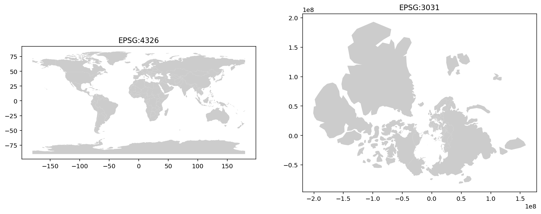
Wait, where’s Antarctica?

If we zoom in on Antarctica, we can see how big a difference these projections make:

antarctica_4326 = world[world['name']=='Antarctica']
antarctica_3031 = world_antarctic[world_antarctic['name']=='Antarctica']

fig, ax = plt.subplots(1,2, figsize=(15,15))
antarctica_4326.plot(ax = ax[0], color='0.8', edgecolor='none')
antarctica_3031.plot(ax = ax[1], color='0.8', edgecolor='none')

ax[0].set_title('EPSG:4326')
ax[1].set_title('EPSG:3031')

Text(0.5, 1.0, 'EPSG:3031')

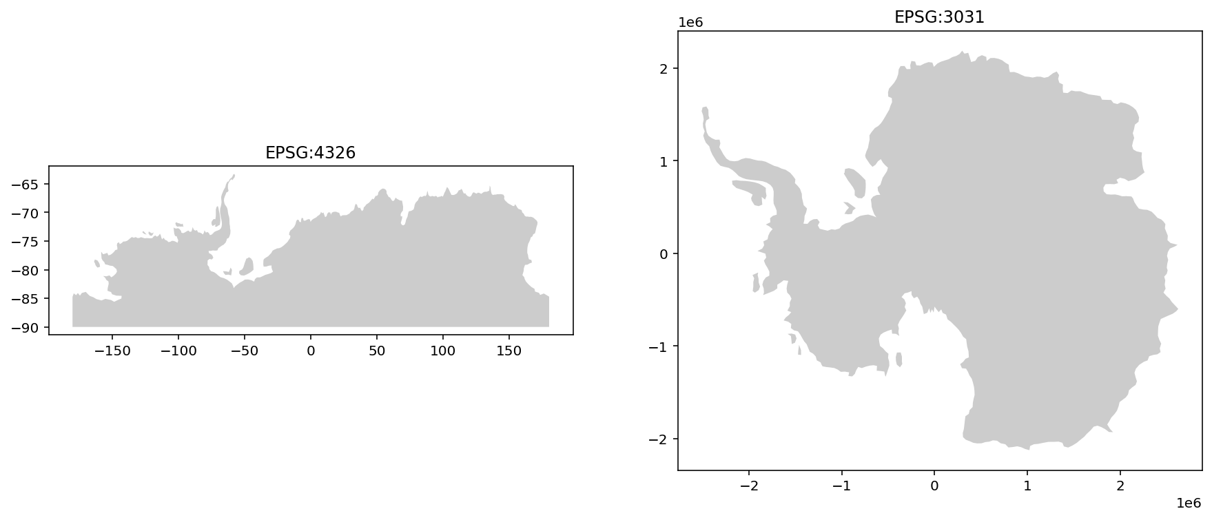
Ahhh Antarctica 🐧

Stereographic projections are common for mapping in polar regions. A lot of legacy data products for both Greenland and Antarctica use polar stereographic projections. Some other polar products, such as NSIDC EASE/EASE-2 grids, are in equal-area projections.

Warning

Stereographic projections are conformal, preserving angles but not distances or areas. Equal-area map projection cannot be conformal, nor can a conformal map projection be equal-area.

Reproject other data

Often you have other data or contextual information that you need to get into your data’s CRS to visualize. For example, you know McMurdo Research Station is at (-77.846 S, 166.676 E). How to we plot this with out using geopandas?

pyproj transform objects can be used to change the Coordinate Reference System of arrays

Important

Note that most Python libraries do NOT check to make sure your data shares the same CRS. Plotting libraries are not “CRS aware” and will happily plot things in incorrect positions. It is up to you to make sure your positions are accurate.

This will transform our latitude and longitude coordinates into coordinates in meters from the map origin

crs4326 = pyproj.CRS.from_epsg(4326)    # WGS84
crs3031 = pyproj.CRS.from_epsg(3031)    # Antarctic Polar Stereographic
transformer = pyproj.Transformer.from_crs(crs4326, crs3031, always_xy=True)

McMurdo = (166.676, -77.846)
McMurdo_3031 = transformer.transform(*McMurdo)

fig, ax = plt.subplots()
antarctica_3031.plot(ax=ax, color='0.8', edgecolor='none')
ax.plot(McMurdo_3031[0], McMurdo_3031[1], 'ko')
ax.set_title(f'McMurdo Station {McMurdo}');

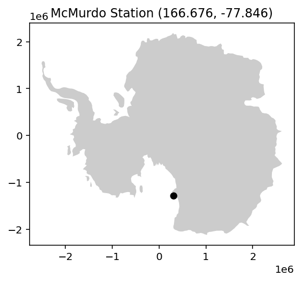
Neat!

Geospatial data comes in two flavors: vector and raster

• Vector data is composed of points, lines, and polygons

• Raster data is composed of individual grid cells

Vector vs. Raster from Planet School

Q: Are you more familiar with using vector or raster data?

Q: Do you more often use GIS software or command-line tools?

ICESat-2

ICESat-2 elevations are in reference to the WGS84 (G1150) ellipsoid.

Important

Recall above we saw EPSG:4326 used “Datum: World Geodetic System 1984 ensemble”, which is common for older or low-accuracy datasets. There are different “realizations” of the WGS84 ellipsoid. The accuracy of your positioning improves when the specific realization, rather than the ensemble, is used. Read more here

ICESat-2 data products also include geoid heights from the EGM2008 geoid. Different ground-based, airborne or satellite-derived elevations may use a separate datum entirely!

Important

Elevations have to be in the same reference frame when comparing heights!

Different datums have different purposes. Heights above mean sea level are needed for ocean and sea ice heights, and are also commonly used for terrestrial mapping (e.g. the elevations of mountains). Ellipsoidal heights are commonly used for estimating land ice height change.

Applying Concepts: ICESat-2

Let’s take what we just learned and apply it to ICESat-2

We’ll download a granule of ICESat-2 ATL06 land ice heights from the National Snow and Ice Data Center (NSIDC). ATL06 is along-track data stored in an HDF5 file with geospatial coordinates latitude and longtude (WGS84). Within an ATL06 file, there are six beam groups (gt1l, gt1r, gt2l, gt2r, gt3l, gt3r) that correspond to the orientation of the beams on the ground.

Note: We just picked a file from random from https://nsidc.org/data/atl06

utilities.attempt_login('urs.earthdata.nasa.gov', retries=5)

<urllib.request.OpenerDirector at 0x7f384d8a07c0>

# query CMR for ATL06 files
ids,urls = utilities.cmr(product='ATL06',release='005',tracks=9,cycles=14,granules=12,verbose=False)
# read ATL06 as in-memory file-like object using xarray
buffer,response_error = utilities.from_nsidc(urls[0])
ds = xr.open_dataset(buffer, group='gt1l/land_ice_segments')
# inspect ATL06 data for beam group
ds

<xarray.Dataset>
Dimensions:                (delta_time: 52945)
Coordinates:
  * delta_time             (delta_time) datetime64[ns] 2021-12-22T21:45:39.28...
    latitude               (delta_time) float64 -79.01 -79.01 ... -68.53 -68.53
    longitude              (delta_time) float64 162.7 162.7 ... 156.8 156.8
Data variables:
    atl06_quality_summary  (delta_time) int8 0 0 0 0 0 0 0 0 ... 1 1 0 0 0 1 1 1
    h_li                   (delta_time) float32 2.842 2.966 2.934 ... -51.76 nan
    h_li_sigma             (delta_time) float32 0.01303 0.01238 ... 0.1829 nan
    segment_id             (delta_time) float64 1.565e+06 ... 1.625e+06
    sigma_geo_h            (delta_time) float32 0.1765 0.1704 ... 5.003 nan
Attributes:
    Description:  The land_ice_height group contains the primary set of deriv...
    data_rate:    Data within this group are sparse.  Data values are provide...

xarray.Dataset

• Dimensions:
  • delta_time: 52945
• Coordinates: (3)
  • delta_time
    (delta_time)
    datetime64[ns]
    2021-12-22T21:45:39.283042640 .....

    contentType :

    referenceInformation

    description :

    Number of GPS seconds since the ATLAS SDP epoch. The ATLAS Standard Data Products (SDP) epoch offset is defined within /ancillary_data/atlas_sdp_gps_epoch as the number of GPS seconds between the GPS epoch (1980-01-06T00:00:00.000000Z UTC) and the ATLAS SDP epoch. By adding the offset contained within atlas_sdp_gps_epoch to delta time parameters, the time in gps_seconds relative to the GPS epoch can be computed.

    long_name :

    Elapsed GPS seconds

    source :

    section 4.4

    standard_name :

    time

    array(['2021-12-22T21:45:39.283042640', '2021-12-22T21:45:39.285857248',
           '2021-12-22T21:45:39.288673408', ..., '2021-12-22T21:48:26.633970320',
           '2021-12-22T21:48:26.636785792', '2021-12-22T21:48:26.681922976'],
          dtype='datetime64[ns]')

  • latitude
    (delta_time)
    float64
    ...

    contentType :

    physicalMeasurement

    description :

    Latitude of segment center, WGS84, North=+,

    long_name :

    Latitude

    source :

    section 3.10

    standard_name :

    latitude

    units :

    degrees_north

    valid_max :

    90.0

    valid_min :

    -90.0

    array([-79.005748, -79.005573, -79.005398, ..., -68.528889, -68.528712,
           -68.525878])

  • longitude
    (delta_time)
    float64
    ...

    contentType :

    physicalMeasurement

    description :

    Longitude of segment center, , WGS84, East=+

    long_name :

    Longitude

    source :

    section 3.10

    standard_name :

    longitude

    units :

    degrees_east

    valid_max :

    180.0

    valid_min :

    -180.0

    array([162.651322, 162.651138, 162.650954, ..., 156.789751, 156.789695,
           156.788747])

• Data variables: (5)
  • atl06_quality_summary
    (delta_time)
    int8
    ...

    contentType :

    qualityInformation

    description :

    The ATL06_quality_summary parameter indicates the best-quality subset of all ATL06 data. A zero in this parameter implies that no data-quality tests have found a problem with the segment, a one implies that some potential problem has been found. Users who select only segments with zero values for this flag can be relatively certain of obtaining high-quality data, but will likely miss a significant fraction of usable data, particularly in cloudy, rough, or low-surface-reflectance conditions.

    flag_meanings :

    best_quality potential_problem

    flag_values :

    [0 1]

    long_name :

    ATL06_Quality_Summary

    source :

    section 4.3

    units :

    1

    valid_max :

    1

    valid_min :

    0

    array([0, 0, 0, ..., 1, 1, 1], dtype=int8)

  • h_li
    (delta_time)
    float32
    ...

    contentType :

    physicalMeasurement

    description :

    Standard land-ice segment height determined by land ice algorithm, corrected for first-photon bias, representing the median- based height of the selected PEs

    long_name :

    Land Ice height

    source :

    section 4.4

    units :

    meters

    array([  2.841663,   2.966382,   2.934198, ..., -51.532295, -51.757175,
                  nan], dtype=float32)

  • h_li_sigma
    (delta_time)
    float32
    ...

    contentType :

    qualityInformation

    description :

    Propagated error due to sampling error and FPB correction from the land ice algorithm

    long_name :

    Expected RMS segment misfit

    source :

    section 4.4

    units :

    meters

    array([0.013026, 0.012383, 0.014085, ..., 0.101088, 0.182853,      nan],
          dtype=float32)

  • segment_id
    (delta_time)
    float64
    ...

    contentType :

    referenceInformation

    description :

    Segment number, counting from the equator. Equal to the segment_id for the second of the two 20m ATL03 segments included in the 40m ATL06 segment

    long_name :

    Reference Point, m

    source :

    section 3.1.2.1

    units :

    1

    array([1565342., 1565343., 1565344., ..., 1624730., 1624731., 1624747.])

  • sigma_geo_h
    (delta_time)
    float32
    ...

    contentType :

    qualityInformation

    description :

    Total vertical geolocation error due to PPD and POD, including the effects of horizontal geolocation error on the segment vertical error.

    long_name :

    Vertical Geolocation Error

    source :

    ATBD Section 3.10

    units :

    meters

    array([0.176499, 0.170433, 0.171702, ..., 5.003703, 5.002903,      nan],
          dtype=float32)

• Attributes: (2)

  Description :

  The land_ice_height group contains the primary set of derived ATL06 products. This includes geolocation, height, and standard error and quality measures for each segment. This group is sparse, meaning that parameters are provided only for pairs of segments for which at least one beam has a valid surface-height measurement.

  data_rate :

  Data within this group are sparse. Data values are provided only for those ICESat-2 20m segments where at least one beam has a valid land ice height measurement.

# For simplicity take first 1000 points into a Geopandas Geodataframe
df = ds.isel(delta_time=slice(0,1000)).to_dataframe()

# NOTE: that the CRS is not propagated by xarray from the HDF5 metadata, so we have to assign it again!
gf = gpd.GeoDataFrame(df, geometry=gpd.points_from_xy(df.longitude, df.latitude), crs='epsg:7661')
gf.head()

	atl06_quality_summary	h_li	h_li_sigma	latitude	longitude	segment_id	sigma_geo_h	geometry
delta_time
2021-12-22 21:45:39.283042640	0	2.841663	0.013026	-79.005748	162.651322	1565342.0	0.176499	POINT (162.65132 -79.00575)
2021-12-22 21:45:39.285857248	0	2.966382	0.012383	-79.005573	162.651138	1565343.0	0.170433	POINT (162.65114 -79.00557)
2021-12-22 21:45:39.288673408	0	2.934198	0.014085	-79.005398	162.650954	1565344.0	0.171702	POINT (162.65095 -79.00540)
2021-12-22 21:45:39.291491568	0	2.991193	0.017458	-79.005223	162.650770	1565345.0	0.181789	POINT (162.65077 -79.00522)
2021-12-22 21:45:39.294311520	0	3.203049	0.015300	-79.005049	162.650588	1565346.0	0.178035	POINT (162.65059 -79.00505)

Visualize with a basemap

import hvplot.pandas # Enable 'hvplot' accessor on Geodataframes for interactive plotting
# Basic plot
# gf.plot.scatter(x='segment_id',y='h_li');
#gf.plot.scatter(x='longitude', y='latitude', c='h_li');

gf.hvplot.points(c='h_li', coastline=True, tiles=True, cmap='viridis', data_aspect=0.1)

Geopandas Reprojection

# As before, we can perform 2D reprojection
gf_3031 = gf.to_crs('epsg:3031')
gf_3031.head()

	atl06_quality_summary	h_li	h_li_sigma	latitude	longitude	segment_id	sigma_geo_h	geometry
delta_time
2021-12-22 21:45:39.283042640	0	2.841663	0.013026	-79.005748	162.651322	1565342.0	0.176499	POINT (357251.485 -1143579.609)
2021-12-22 21:45:39.285857248	0	2.966382	0.012383	-79.005573	162.651138	1565343.0	0.170433	POINT (357260.883 -1143596.736)
2021-12-22 21:45:39.288673408	0	2.934198	0.014085	-79.005398	162.650954	1565344.0	0.171702	POINT (357270.271 -1143613.868)
2021-12-22 21:45:39.291491568	0	2.991193	0.017458	-79.005223	162.650770	1565345.0	0.181789	POINT (357279.638 -1143631.012)
2021-12-22 21:45:39.294311520	0	3.203049	0.015300	-79.005049	162.650588	1565346.0	0.178035	POINT (357288.984 -1143648.167)

Copernicus DEM

Let’s compare ICESat-2 elevations against a public, gridded global digital elevation model (DEM), the Copernicus DEM. Just as Geopandas adds CRS-aware capabilities to Dataframes, RioXarray adds CRS-aware functions to XArray multidimensional arrays (e.g. sets of images).

daC = rioxarray.open_rasterio('https://opentopography.s3.sdsc.edu/raster/COP30/COP30_hh.vrt', 
                              chunks=True, # ensure we use dask to only read metadata
                             )


# Crop by Bounding box of all the ATL06 points
minx, miny, maxx, maxy = gf.cascaded_union.envelope.bounds
daC = daC.rio.clip_box(minx, miny, maxx, maxy)
daC

<xarray.DataArray (band: 1, y: 631, x: 636)>
dask.array<copy, shape=(1, 631, 636), dtype=float32, chunksize=(1, 631, 636), chunktype=numpy.ndarray>
Coordinates:
  * band         (band) int64 1
  * x            (x) float64 162.5 162.5 162.5 162.5 ... 162.7 162.7 162.7 162.7
  * y            (y) float64 -78.83 -78.83 -78.83 ... -79.01 -79.01 -79.01
    spatial_ref  int64 0
Attributes:
    scale_factor:  1.0
    add_offset:    0.0

xarray.DataArray

• band: 1
• y: 631
• x: 636

• dask.array<chunksize=(1, 631, 636), meta=np.ndarray>

  Array Chunk Bytes 1.53 MiB 1.53 MiB Shape (1, 631, 636) (1, 631, 636) Count 24637 Tasks 1 Chunks Type float32 numpy.ndarray

• Coordinates: (4)
  • band
    (band)
    int64
    1

    array([1])

  • x
    (x)
    float64
    162.5 162.5 162.5 ... 162.7 162.7

    axis :

    X

    long_name :

    longitude

    standard_name :

    longitude

    units :

    degrees_east

    array([162.474861, 162.475139, 162.475417, ..., 162.650694, 162.650972,
           162.65125 ])

  • y
    (y)
    float64
    -78.83 -78.83 ... -79.01 -79.01

    axis :

    Y

    long_name :

    latitude

    standard_name :

    latitude

    units :

    degrees_north

    array([-78.830833, -78.831111, -78.831389, ..., -79.005278, -79.005556,
           -79.005833])

  • spatial_ref
    ()
    int64
    0

    crs_wkt :

    GEOGCS["WGS 84",DATUM["WGS_1984",SPHEROID["WGS 84",6378137,298.257223563,AUTHORITY["EPSG","7030"]],AUTHORITY["EPSG","6326"]],PRIMEM["Greenwich",0,AUTHORITY["EPSG","8901"]],UNIT["degree",0.0174532925199433,AUTHORITY["EPSG","9122"]],AXIS["Latitude",NORTH],AXIS["Longitude",EAST],AUTHORITY["EPSG","4326"]]

    semi_major_axis :

    6378137.0

    semi_minor_axis :

    6356752.314245179

    inverse_flattening :

    298.257223563

    reference_ellipsoid_name :

    WGS 84

    longitude_of_prime_meridian :

    0.0

    prime_meridian_name :

    Greenwich

    geographic_crs_name :

    WGS 84

    grid_mapping_name :

    latitude_longitude

    spatial_ref :

    GEOGCS["WGS 84",DATUM["WGS_1984",SPHEROID["WGS 84",6378137,298.257223563,AUTHORITY["EPSG","7030"]],AUTHORITY["EPSG","6326"]],PRIMEM["Greenwich",0,AUTHORITY["EPSG","8901"]],UNIT["degree",0.0174532925199433,AUTHORITY["EPSG","9122"]],AXIS["Latitude",NORTH],AXIS["Longitude",EAST],AUTHORITY["EPSG","4326"]]

    GeoTransform :

    162.4747222222222 0.00027777777777776385 0.0 -78.83069444444446 0.0 -0.0002777777777777507

    array(0)

• Attributes: (2)

  scale_factor :

  1.0

  add_offset :

  0.0

# enable hvplot accessor on xarray datasets
daC.squeeze('band').hvplot.image(rasterize=True, 
                                 cmap='viridis', 
                                 title='Copernicus 30m DEM')

# Like Geopandas, Rioxarray handles CRS information for gridded arrays!
daC.rio.crs 

CRS.from_epsg(4326)

# Some geospatial rasters fail to include metadata about the NaN values
# This ensures Python recognizes values as NaNs, but when writing to a TIF file those values are assigned -32768.0
daC.rio.write_nodata(-32768.0, encoded=True, inplace=True)

<xarray.DataArray (band: 1, y: 631, x: 636)>
dask.array<copy, shape=(1, 631, 636), dtype=float32, chunksize=(1, 631, 636), chunktype=numpy.ndarray>
Coordinates:
  * band         (band) int64 1
  * x            (x) float64 162.5 162.5 162.5 162.5 ... 162.7 162.7 162.7 162.7
  * y            (y) float64 -78.83 -78.83 -78.83 ... -79.01 -79.01 -79.01
    spatial_ref  int64 0
Attributes:
    scale_factor:  1.0
    add_offset:    0.0

xarray.DataArray

• band: 1
• y: 631
• x: 636

• dask.array<chunksize=(1, 631, 636), meta=np.ndarray>

  Array Chunk Bytes 1.53 MiB 1.53 MiB Shape (1, 631, 636) (1, 631, 636) Count 24637 Tasks 1 Chunks Type float32 numpy.ndarray

• Coordinates: (4)
  • band
    (band)
    int64
    1

    array([1])

  • x
    (x)
    float64
    162.5 162.5 162.5 ... 162.7 162.7

    axis :

    X

    long_name :

    longitude

    standard_name :

    longitude

    units :

    degrees_east

    array([162.474861, 162.475139, 162.475417, ..., 162.650694, 162.650972,
           162.65125 ])

  • y
    (y)
    float64
    -78.83 -78.83 ... -79.01 -79.01

    axis :

    Y

    long_name :

    latitude

    standard_name :

    latitude

    units :

    degrees_north

    array([-78.830833, -78.831111, -78.831389, ..., -79.005278, -79.005556,
           -79.005833])

  • spatial_ref
    ()
    int64
    0

    crs_wkt :

    GEOGCS["WGS 84",DATUM["WGS_1984",SPHEROID["WGS 84",6378137,298.257223563,AUTHORITY["EPSG","7030"]],AUTHORITY["EPSG","6326"]],PRIMEM["Greenwich",0,AUTHORITY["EPSG","8901"]],UNIT["degree",0.0174532925199433,AUTHORITY["EPSG","9122"]],AXIS["Latitude",NORTH],AXIS["Longitude",EAST],AUTHORITY["EPSG","4326"]]

    semi_major_axis :

    6378137.0

    semi_minor_axis :

    6356752.314245179

    inverse_flattening :

    298.257223563

    reference_ellipsoid_name :

    WGS 84

    longitude_of_prime_meridian :

    0.0

    prime_meridian_name :

    Greenwich

    geographic_crs_name :

    WGS 84

    grid_mapping_name :

    latitude_longitude

    spatial_ref :

    GEOGCS["WGS 84",DATUM["WGS_1984",SPHEROID["WGS 84",6378137,298.257223563,AUTHORITY["EPSG","7030"]],AUTHORITY["EPSG","6326"]],PRIMEM["Greenwich",0,AUTHORITY["EPSG","8901"]],UNIT["degree",0.0174532925199433,AUTHORITY["EPSG","9122"]],AXIS["Latitude",NORTH],AXIS["Longitude",EAST],AUTHORITY["EPSG","4326"]]

    GeoTransform :

    162.4747222222222 0.00027777777777776385 0.0 -78.83069444444446 0.0 -0.0002777777777777507

    array(0)

• Attributes: (2)

  scale_factor :

  1.0

  add_offset :

  0.0

RioXarray Reprojection

Warning

Unfortunately, data files alone do not always include the full CRS information! For example, reading the documentation about copernicus DEM we see Vertical Coordinates: EGM2008 [EPSG: 3855]. These elevations are “geoid” heights. With respect to the EGM2008 model.

We can still reproject this array as we did before, using only horizontal transformations:

from rasterio.enums import Resampling

# reprojecting to a new grid requires an interpolation method
# here it will resample using bilinear interpolation
daC_3031 = daC.rio.reproject('EPSG:3031',
                             resampling=Resampling.bilinear, 
                            )

#daC_3031.plot(); #static matplotlib
daC_3031.squeeze('band').hvplot.image(rasterize=True,
                                      data_aspect=1,
                                      cmap='viridis',
                                      title='COP30 DEM EPSG:3031',
                                     )

3D Reference Systems and Datums

Coordinates are defined to be in reference to the origins of the coordinate system

• Horizontally, coordinates are in reference to the Equator and the Prime Meridian

• Vertically, heights are in reference to a datum

Two common vertical datums are the reference ellipsoid and the reference geoid.

What are they and what is the difference?

• To first approximation, the Earth is a sphere (🐄) with a radius of 6371 kilometers.

• To a better approximation, the Earth is a slightly flattened ellipsoid with the polar axis 22 kilometers shorter than the equatorial axis.

• To an even better approximation, the Earth’s shape can be described using a reference geoid, which undulates 10s of meters above and below the reference ellipsoid. The difference in height between the ellipsoid and the geoid are known as geoid heights.

The geoid is an equipotential surface, perpendicular to the force of gravity at all points and with a constant geopotential. Reference ellipsoids and geoids are both created to largely coincide with mean sea level if the oceans were at rest.

An ellipsoid can be considered a simplification of a geoid.

PROJ hosts grids for shifting both the horizontal and vertical datum, such as gridded EGM2008 geoid height values

Additional geoid height values can be calculated at the International Centre for Global Earth Models (ICGEM)

Vertically exaggerated, the Earth is sort of like a potato 🥔

PROJ Reprojection pipelines

We can examine details of converting any projection to another with PROJ. Specific vertical datums also have EPSG codes so you can refer to horizontal and vertical coordinates separately with a compound CRS. Below is the recipe for converting the Copernicus DEM (geoid) to ellipsoidal heights matching ATL06. Note that we require the use of a precomputed vertical shift grid (pictured above).

!projinfo -s EPSG:4326+3855 -t EPSG:7661 -o PROJ --hide-ballpark --spatial-test intersects

Candidate operations found: 1
-------------------------------------
Operation No. 1:

unknown id, Inverse of WGS 84 to EGM2008 height (1) + WGS 84 to WGS 84 (G1150), 3 m, World., at least one grid missing

PROJ string:
+proj=pipeline
  +step +proj=axisswap +order=2,1
  +step +proj=unitconvert +xy_in=deg +xy_out=rad
  +step +proj=vgridshift +grids=us_nga_egm08_25.tif +multiplier=1
  +step +proj=unitconvert +xy_in=rad +xy_out=deg
  +step +proj=axisswap +order=2,1

Grid us_nga_egm08_25.tif needed but not found on the system. Can be obtained at https://cdn.proj.org/us_nga_egm08_25.tif

Numba: Attempted to fork from a non-main thread, the TBB library may be in an invalid state in the child process.

Geospatial Data Abstraction Library (GDAL)

If you need to do 3D transformations, GDAL is a great solution! It uses PROJ behind the scenes

The Geospatial Data Abstraction Library (GDAL/OGR) is a powerful piece of software.

It can read, write and query a wide variety of raster and vector geospatial data formats, transform the coordinate system of images, and manipulate other forms of geospatial data.

It is the backbone of a large suite of geospatial libraries and programs.

There are a number of wrapper libraries (e.g. rasterio, rioxarray, shapely, fiona) that provide more user-friendly interfaces with GDAL functionality.

Similar to pyproj CRS objects, GDAL SpatialReference functions can provide a lot of information about a particular Coordinate Reference System

Geoid -> Ellipsoid height

We’ll use GDAL to reproject a subset of the Copernicus DEM into EPSG:7661 (apply a vertical shift grid)

ulx, lry, lrx, uly = gf.cascaded_union.envelope.bounds
print('lower right', lrx, lry)
print('upper left', ulx, uly)

lower right 162.65132243386927 -79.00574767564308
upper left 162.47496995103063 -78.83096643118282

# Download subset locally
infile = '/vsicurl/https://opentopography.s3.sdsc.edu/raster/COP30/COP30_hh.vrt'
outfile = '/tmp/COP30_subset.tif'

!GDAL_DISABLE_READDIR_ON_OPEN=EMPTY_DIR gdal_translate -projwin {ulx} {uly} {lrx} {lry} {infile} {outfile}

Numba: Attempted to fork from a non-main thread, the TBB library may be in an invalid state in the child process.

Input file size is 1296005, 626400

0

...10...20...30...40...50...60...70...80...90...100 - done.

Note

Whenever conducting complicated transformations it can be helpful to print ‘DEBUG’ messages to ensure libraries are doing what you expect behind the scenes

In the following cell, we see GDAL tries to find the necessary vertical shift grid files locally, doesn’t find it, so the automatically retrieves it from a server:

!CPL_DEBUG=ON PROJ_DEBUG=2 gdalwarp -s_srs EPSG:4326+3855 -t_srs EPSG:7661 /tmp/COP30_subset.tif /tmp/cop_7661.tif

PROJ: pj_open_lib(proj.db): call fopen(/usr/share/miniconda3/envs/hackweek/share/proj/proj.db) - succeeded
GDAL: GDALOpen(/tmp/COP30_subset.tif, this=0x55dcefe3ef50) succeeds as GTiff.
GDAL: Using GTiff driver

PROJ: pj_open_lib(proj.ini): call fopen(/usr/share/miniconda3/envs/hackweek/share/proj/proj.ini) - succeeded
GDAL: Computing area of interest: 162.475, -79.0054, 162.651, -78.8307
OGRCT: Wrap source at 162.563.
PROJ: pj_open_lib(us_nga_egm08_25.tif): call fopen(/usr/share/miniconda3/envs/hackweek/share/proj/us_nga_egm08_25.tif) - failed
PROJ: pj_open_lib(egm08_25.gtx): call fopen(/usr/share/miniconda3/envs/hackweek/share/proj/egm08_25.gtx) - failed

Numba: Attempted to fork from a non-main thread, the TBB library may be in an invalid state in the child process.

PROJ: Using https://cdn.proj.org/us_nga_egm08_25.tif

PROJ: pj_open_lib(us_nga_egm08_25.tif): call fopen(/usr/share/miniconda3/envs/hackweek/share/proj/us_nga_egm08_25.tif) - failed
PROJ: pj_open_lib(egm08_25.gtx): call fopen(/usr/share/miniconda3/envs/hackweek/share/proj/egm08_25.gtx) - failed
PROJ: Using https://cdn.proj.org/us_nga_egm08_25.tif

Creating output file that is 635P x 629L.
GDAL: GDALDriver::Create(GTiff,/tmp/cop_7661.tif,635,629,1,Float32,(nil))
Processing /tmp/COP30_subset.tif [1/1] : 0WARP: Copying metadata from first source to destination dataset
GTiff: ScanDirectories()
GDAL: GDALDefaultOverviews::OverviewScan()
GDALWARP: Defining SKIP_NOSOURCE=YES
PROJ: Using coordinate operation WGS 84 to EGM2008 height (1)
PROJ: pj_open_lib(us_nga_egm08_25.tif): call fopen(/usr/share/miniconda3/envs/hackweek/share/proj/us_nga_egm08_25.tif) - failed
PROJ: pj_open_lib(egm08_25.gtx): call fopen(/usr/share/miniconda3/envs/hackweek/share/proj/egm08_25.gtx) - failed
PROJ: Using https://cdn.proj.org/us_nga_egm08_25.tif

PROJ: Using coordinate operation WGS 84 to EGM2008 height (1)
PROJ: pj_open_lib(us_nga_egm08_25.tif): call fopen(/usr/share/miniconda3/envs/hackweek/share/proj/us_nga_egm08_25.tif) - failed
PROJ: pj_open_lib(egm08_25.gtx): call fopen(/usr/share/miniconda3/envs/hackweek/share/proj/egm08_25.gtx) - failed
PROJ: Using https://cdn.proj.org/us_nga_egm08_25.tif
GDAL: GDAL_CACHEMAX = 347 MB
GDAL: GDALWarpKernel()::GWKNearestNoMasksOrDstDensityOnlyFloat() Src=0,0,635x629 Dst=0,0,635x629
...10.

..20...30...40...50.

..60...70...80...90

...100 - done.
GDAL: Flushing dirty blocks: 0...10...20...30...40...50...60...70...80...90...100 - done.
GTiff: Adjusted bytes to write from 7620 to 5080.
GDAL: GDALClose(/tmp/cop_7661.tif, this=0x55dcf065d9c0)
GDAL: GDALClose(/tmp/COP30_subset.tif, this=0x55dcefe3ef50)

da = rioxarray.open_rasterio('/tmp/cop_7661.tif')
da.rio.crs

CRS.from_epsg(7661)

da.squeeze('band').hvplot.image(x='x', y='y', 
                               rasterize=True,
                               title='COP30 DEM (EPSG:7661)'
                              )

Summary

🎉 Congrats! You’ve made it through the tutorial! You have successfully reprojected geospatial vector data (country polygons, IS2 ATL06) and raster imagery (Copernicus DEM). You’ve seen how to perform both 2D horizontal reprojections with both GeoPandas and RioXarray, and we looked into more advanced 3D reprojection pipelines with PROJ and GDAL.

A good next step would be to make some plots comparing elevation values! Have a look at documentation on reprojecting different rasters to exactly the same grid, and sampling rasters at points. Below we include additional references, and we’ve also put together a second notebook that goes into some of these topics in more depth.

References

There are entire graduate-level courses and great educational material to learn more about these topics. We recommend checking out:

• PennState GPS & GNSS for Geospatial Professionals

• UW Geospatial Data Analaysis with Python

• Qinsy Geodetic Documentation

previous

Alien exercise

next

Geospatial Transformations In-depth