.ipynb .pdf

repository open issue suggest edit

Binder

Contents

Data integration with ICESat-2 - Part II

Credits

• Zach Fair

• Ian Joughin

• Tasha Snow

Learning Objectives

Goals

• Access NSIDC data sets and acquire IS-2 using icepyx

• Analyze point and raster data together with IS-2

• Advanced visualizations of multiple datasets

For this tutorial, feel free to run the code along with us as we live code by downsizing the zoom window and splitting your screen (or using two screens). Or you can simply watch the zoom walkthrough. Don’t worry if you fall behind on the code. The notebook is standalone and you can easily run the code at your own pace another time to catch anything you missed.

Python environment

GrIMP libraries

This notebook makes use of two packages for working with data from the Greenland Ice Mapping Project (GrIMP) that are stored remotely at NSIDC. These packages are:

• grimpfunc: Code for searching NISDC catalog for GrIMP data, subsetting the data, and working with flowlines.

• nisardev: Classes for working with velocity and image data.

import numpy as np
import nisardev as nisar
import os
import matplotlib.colors as mcolors
import grimpfunc as grimp
import matplotlib.pyplot as plt
import geopandas as gpd
import pandas as pd
from datetime import datetime
import numpy as np
import xarray as xr
import importlib
import requests
import pyproj
from mpl_toolkits.axes_grid1.inset_locator import inset_axes
import panel
from dask.diagnostics import ProgressBar
import h5py
import random

import ipyleaflet
from ipyleaflet import Map,GeoData,LegendControl,LayersControl,Rectangle,basemaps,basemap_to_tiles,TileLayer,SplitMapControl,Polygon,Polyline

import ipywidgets
import datetime
import re

ProgressBar().register()
panel.extension()

Sometimes the above cell will return an error about a missing module. If this happens, try restarting the kernel and re-running the above cells.

NSIDC Login

For remote access to the velocity data at NSIDC, run these cells to login with your NASA EarthData Login (see NSIDCLoginNotebook for further details). These cells can skipped if all data are being accessed locally. First define where the cookie files need for login are saved.

These environment variables are used by GDAL for remote data access via vsicurl.

env = dict(GDAL_HTTP_COOKIEFILE=os.path.expanduser('~/.grimp_download_cookiejar.txt'),
            GDAL_HTTP_COOKIEJAR=os.path.expanduser('~/.grimp_download_cookiejar.txt'))
os.environ.update(env)

Now enter credentials, which will create the cookie files above as well as .netrc file with the credentials.

#!rm ~/.netrc
myLogin = grimp.NASALogin()
myLogin.view()

Getting login from ~/.netrc

Already logged in. Proceed.

Load glacier termini

In this section we will read shapefiles stored remotely at NSIDC.

The first step is to get the urls for the files in the NSDIC catalog.

myTerminusUrls = grimp.cmrUrls(mode='terminus')  # mode image restricts search to the image products
myTerminusUrls.initialSearch();

Using the myTerminusUrls.getURLS() method to return the urls for the shape files, read in termini and store in a dict, myTermini, by year.

myTermini = {}
for url in myTerminusUrls.getURLS():
    year = os.path.basename(url).split('_')[1]  # Extract year from name
    myTermini[year] = gpd.read_file(f'/vsicurl/&url={url}')  # Add terminus to data frame
    print(f'/vsicurl/&url={url}')

/vsicurl/&url=https://n5eil01u.ecs.nsidc.org/DP4/MEASURES/NSIDC-0642.002/2000.09.30/termini_2000_2001_v02.0.shp

/vsicurl/&url=https://n5eil01u.ecs.nsidc.org/DP4/MEASURES/NSIDC-0642.002/2005.12.24/termini_2005_2006_v02.0.shp

/vsicurl/&url=https://n5eil01u.ecs.nsidc.org/DP4/MEASURES/NSIDC-0642.002/2007.01.06/termini_2006_2007_v02.0.shp

/vsicurl/&url=https://n5eil01u.ecs.nsidc.org/DP4/MEASURES/NSIDC-0642.002/2007.11.22/termini_2007_2008_v02.0.shp

/vsicurl/&url=https://n5eil01u.ecs.nsidc.org/DP4/MEASURES/NSIDC-0642.002/2009.01.04/termini_2008_2009_v02.0.shp

/vsicurl/&url=https://n5eil01u.ecs.nsidc.org/DP4/MEASURES/NSIDC-0642.002/2013.01.15/termini_2012_2013_v02.0.shp

/vsicurl/&url=https://n5eil01u.ecs.nsidc.org/DP4/MEASURES/NSIDC-0642.002/2015.02.07/termini_2014_2015_v02.0.shp

/vsicurl/&url=https://n5eil01u.ecs.nsidc.org/DP4/MEASURES/NSIDC-0642.002/2016.02.02/termini_2015_2016_v02.0.shp

/vsicurl/&url=https://n5eil01u.ecs.nsidc.org/DP4/MEASURES/NSIDC-0642.002/2017.02.01/termini_2016_2017_v02.0.shp

/vsicurl/&url=https://n5eil01u.ecs.nsidc.org/DP4/MEASURES/NSIDC-0642.002/2018.02.02/termini_2017_2018_v02.0.shp

/vsicurl/&url=https://n5eil01u.ecs.nsidc.org/DP4/MEASURES/NSIDC-0642.002/2019.02.03/termini_2018_2019_v02.0.shp

/vsicurl/&url=https://n5eil01u.ecs.nsidc.org/DP4/MEASURES/NSIDC-0642.002/2020.02.04/termini_2019_2020_v02.0.shp

/vsicurl/&url=https://n5eil01u.ecs.nsidc.org/DP4/MEASURES/NSIDC-0642.002/2021.02.04/termini_2020_2021_v02.0.shp

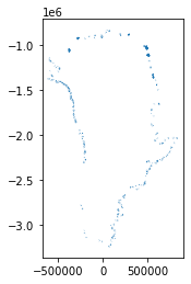
myTermini['2000'].plot()

<AxesSubplot:>

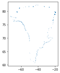
for year in myTermini:
    myTermini[year] = myTermini[year].to_crs('EPSG:4326') # to lat/lon
myTermini['2000'].plot()  

<AxesSubplot:>

Flowlines

In this section we will work with a two collections of flowlines from Felikson et al., 2020. The full set of flowines for all of Greenland can be downloaded from Zenodo.

The data are stored in the subdirectory shpfiles and can be read as follows:

glaciers = {}
for i in range(1, 3):
    glaciers[f'000{i}'] = gpd.read_file(f'shpfiles/glacier000{i}.shp').to_crs('EPSG:4326');

Note this is the same procedure as for the termini, except we are using a filename instead of a url.

ICESat-2 ATL06

Now that we have the flowlines and termini, we are going to plot these alongside the ICESat-2 and ATM tracks. Remember the data we worked with yesterday? Here we are going to use that again for this mappinp project.

# Load the ICESat-2 data
is2_file = 'processed_ATL06_20190420093051_03380303_005_01_full.h5'
with h5py.File(is2_file, 'r') as f:
    is2_gt2r = pd.DataFrame(data={'lat': f['gt2r/land_ice_segments/latitude'][:],
                                  'lon': f['gt2r/land_ice_segments/longitude'][:],
                                  'elev': f['gt2r/land_ice_segments/h_li'][:]}) # Central weak beam
    is2_gt2l = pd.DataFrame(data={'lat': f['gt2l/land_ice_segments/latitude'][:],
                                  'lon': f['gt2l/land_ice_segments/longitude'][:],
                                  'elev': f['gt2l/land_ice_segments/h_li'][:]}) # Central strong beam
    
# Load the ATM data
atm_file = 'ILATM2_20190506_151600_smooth_nadir3seg_50pt.csv'
atm_l2 = pd.read_csv(atm_file)

# Look only at the nadir track
atm_l2 = atm_l2[atm_l2['Track_Identifier']==0]

# Change the longitudes to be consistent with ICESat-2
atm_l2['Longitude(deg)'] -= 360

Next the data are subsetted to the range of ATM latitudes.

# Subset the ICESat-2 data to the ATM latitudes
is2_gt2r = is2_gt2r[(is2_gt2r['lat']<atm_l2['Latitude(deg)'].max()) & (is2_gt2r['lat']>atm_l2['Latitude(deg)'].min())]
is2_gt2l = is2_gt2l[(is2_gt2l['lat']<atm_l2['Latitude(deg)'].max()) & (is2_gt2l['lat']>atm_l2['Latitude(deg)'].min())]

Plot lidar tracks, flowlines and termini

Checking everything looks good before analysis by plotting the data over imagery rendered via ipyleaflet.

center = [69.2, -50]
zoom = 8

mapdt1 = '2019-05-06'

m = Map(basemap=basemap_to_tiles(basemaps.NASAGIBS.ModisAquaTrueColorCR, mapdt1),center=center,zoom=zoom)

gt2r_line = Polyline(
    locations=[
        [is2_gt2r['lat'].min(), is2_gt2r['lon'].max()],
        [is2_gt2r['lat'].max(), is2_gt2r['lon'].min()]
    ],
    color="green" ,
    fill=False
)
m.add_layer(gt2r_line)

gt2l_line = Polyline(
    locations=[
        [is2_gt2l['lat'].min(), is2_gt2l['lon'].max()],
        [is2_gt2l['lat'].max(), is2_gt2l['lon'].min()]
    ],
    color="green" ,
    fill=False
)
m.add_layer(gt2l_line)

atm_line = Polyline(
    locations=[
        [atm_l2['Latitude(deg)'].min(), atm_l2['Longitude(deg)'].max()],
        [atm_l2['Latitude(deg)'].max(), atm_l2['Longitude(deg)'].min()]
    ],
    color="orange" ,
    fill=False
)
m.add_layer(atm_line)
legend = LegendControl({'ICESat-2':'green','ATM':'orange'}, name = 'Lidar', position="topleft")
m.add_control(legend)

tLegend = {}
for i in range(3, 5):
    for key in myTermini:
        # Create list of lat/lon pairs
        r = lambda: random.randint(0,255)
        cr = '#%02X%02X%02X' % (r(),r(),r())
        term_coords = [[[xy[1],xy[0]] for xy in geom.coords] for geom in myTermini[key].loc[myTermini[key]['Glacier_ID'] == i].geometry]
        term_data = Polyline(locations=term_coords, weight=2, color=cr, fill=False)
        m.add_layer(term_data)
        tLegend[key] = cr
legend = LegendControl(tLegend, name="Terminus", position="topright")
m.add_control(legend)

for glacier in glaciers:
    gl_data = GeoData(geo_dataframe = glaciers[glacier],
                   style={'color': 'black', 'weight':1.0},
                   name = f'{glacier}')
    m.add_layer(gl_data)
    
m.add_control(LayersControl())

m

Plot Flowines Using Remote Greenland Ice Mapping Project Data

ICESat measures thinning and thickening, which often is driven by changes in the flow of the glacier.

Thus, to understand whether elevation change is driven by ice dynamics or changes in surface mass balance (net melting and snowfall), we need to look at how the flow velocity is evolving with time.

This section demonstrates how Greenland Ice Mapping Project (GrIMP) data can be remotely accessed. As an example, will used flowlines from Felikson et al., 2020 distributed via Zenodo.

Here we will use:

• grimp.Flowlines to read, manipulate, and store the flowlines data;

• grimp.cmrUrls to search the NISDC catalog; and

• nisar.nisarVelSeries to build a time-dependent stack of velocity data, which be plotted, interpolated etc.

Read Shapefiles

In the examples presented here we will use glaciers 1 & 2 in the Felikson data base, Felikson et al., 2020, which were retrieved from Zenodo.

Each glacier’s flowlines are used to create grimp.Flowlines instances, which are saved in a dictionary, myFlowlines with glacier id: ‘0001’ and ‘0002’.

Each Flowlines read a set of flowlines for each glacier and stores in a dictionary of myFlowlines.flowlines. The code to do this looks something like:

    flowlines = {}
    shapeTable = gpd.read_file(shapefile)
    for index, row in shapeTable.iterrows():  # loop over features
        fl = {}  # New Flowline
        fl['x'], fl['y'] = np.array([c for c in row['geometry'].coords]).transpose()
        fl['d'] = computeDistance(fl['x'], fl['y'])
        flowlines[row['flowline']] = fl

For further detail, see the full class definition

To limit the plots to the downstream regions, the flowlines are all truncated to a length of 50km.

Within each myFlowines entry (a grimp.Flowlines instance), the individual flowlines are maintained as a dictionary myFlowlines['glacierId'].flowlines.

myShapeFiles = [f'./shpfiles/glacier000{i}.shp' for i in range(1, 3)] # Build list of shape file names
myFlowlines = {x[-8:-4]: grimp.Flowlines(shapefile=x, name=x[-8:-4], length=50e3) for x in myShapeFiles} 
myFlowlines

{'0001': <grimpfunc.Flowlines.Flowlines at 0x7f2bacd10ee0>,
 '0002': <grimpfunc.Flowlines.Flowlines at 0x7f2bacd3ec10>}

Each flowline is indexed as shown here:

myFlowlines['0001'].flowlines.keys()

dict_keys(['03', '04', '05', '06', '07', '08'])

The data for the flow line is simple, just x, y polar stereographic coordinates (EPSG=3413) and the distance, d, from the start of the flowline.

myFlowlines['0001'].flowlines['03'].keys()

dict_keys(['x', 'y', 'd'])

These coordinates for a given index can be returned as myFlowlines['0001'].xym(index='03') or myFlowlines['0001'].xykm(index='03') depending on whether m or km are preferred.

The area of interest can be defined as the union of the bounds for all of the flowlines computed as shown below along with the unique set of flowline IDs across all glaciers. We will use the bounding box below to subset the data.

myBounds = {'minx': 1e9, 'miny': 1e9, 'maxx': -1e9, 'maxy': -1e9}  # Initial bounds to force reset
flowlineIDs = []  # 
for myKey in myFlowlines:
    # Get bounding box for flowlines
    flowlineBounds = myFlowlines[myKey].bounds
    # Merge with prior bounds
    myBounds = myFlowlines[myKey].mergeBounds(myBounds, flowlineBounds)
    # Get the flowline ids
    flowlineIDs.append(myFlowlines[myKey].flowlineIDs())
# Get the unique list of flowlines ids (used for legends later)
flowlineIDs = np.unique(flowlineIDs)
print(myBounds)
print(flowlineIDs)

{'minx': -220000.0, 'miny': -2314100.0, 'maxx': -127800.0, 'maxy': -2219100.0}
['03' '04' '05' '06' '07' '08']

Search Catalog for Velocity Data

We now need to locate velocity data from the GrIMP data set. For this exercise, we will focus on the annual velocity maps of Greenland. To do this, we will use the grimp.cmrUrls tool, which will do a GUI based search of NASA’s Common Metadata Repository (CMR). Search parameters can be passe directly to initialSearch method to perform the search.

myUrls = grimp.cmrUrls(mode='subsetter', verbose=True)  # nisar mode excludes image and tsx products and allows only one product type at a time
myUrls.initialSearch(product='NSIDC-0725')

https://cmr.earthdata.nasa.gov/search/granules.json?provider=NSIDC_ECS&sort_key[]=start_date&sort_key[]=producer_granule_id&scroll=false&page_size=2000&page_num=1&short_name=NSIDC-0725&version=3&temporal[]=2000-01-01T00:00:01Z,2022-04-14T00:23:59&bounding_box[]=-75.00,60.00,-5.00,82.00&producer_granule_id[]=*&options[producer_granule_id][pattern]=true

The verbose flag causes the CMR search string to be printed. The search basically works by a) reading the parameters from the search panel (e.g., product, date, etc) and creating a search string, which returns the search result.

response = requests.get('https://cmr.earthdata.nasa.gov/search/granules.json?provider=NSIDC_ECS&sort_key[]=start_date&sort_key[]='
                        'producer_granule_id&scroll=false&page_size=2000&page_num=1&short_name=NSIDC-0725&version=3&temporal[]='
                        '2000-01-01T00:00:01Z,2022-03-10T00:23:59&bounding_box[]=-75.00,60.00,-5.00,82.00&producer_granule_id[]='
                        '*&options[producer_granule_id][pattern]=true')
search_results = response.json()
search_results;

Under the hood, the cmrUrls code can filter the json to get a list of urls:

myUrls.getURLS()

https://cmr.earthdata.nasa.gov/search/granules.json?provider=NSIDC_ECS&sort_key[]=start_date&sort_key[]=producer_granule_id&scroll=false&page_size=2000&page_num=1&short_name=NSIDC-0725&version=3&temporal[]=2000-01-01T00:00:01Z,2022-04-14T00:23:59&bounding_box[]=-75.00,60.00,-5.00,82.00&producer_granule_id[]=*&options[producer_granule_id][pattern]=true

['https://n5eil01u.ecs.nsidc.org/DP4/MEASURES/NSIDC-0725.003/2014.12.01/GL_vel_mosaic_Annual_01Dec14_30Nov15_vv_v03.0.tif',
 'https://n5eil01u.ecs.nsidc.org/DP4/MEASURES/NSIDC-0725.003/2015.12.01/GL_vel_mosaic_Annual_01Dec15_30Nov16_vv_v03.0.tif',
 'https://n5eil01u.ecs.nsidc.org/DP4/MEASURES/NSIDC-0725.003/2016.12.01/GL_vel_mosaic_Annual_01Dec16_30Nov17_vv_v03.0.tif',
 'https://n5eil01u.ecs.nsidc.org/DP4/MEASURES/NSIDC-0725.003/2017.12.01/GL_vel_mosaic_Annual_01Dec17_30Nov18_vv_v03.0.tif',
 'https://n5eil01u.ecs.nsidc.org/DP4/MEASURES/NSIDC-0725.003/2018.12.01/GL_vel_mosaic_Annual_01Dec18_30Nov19_vv_v03.0.tif',
 'https://n5eil01u.ecs.nsidc.org/DP4/MEASURES/NSIDC-0725.003/2019.12.01/GL_vel_mosaic_Annual_01Dec19_30Nov20_vv_v03.0.tif']

Load the Velocity Data

GrIMP produces full Greenland velocity maps. Collectively, there are more than 400 full Greenland maps, totalling several hundred GB of data, which may be more than a user interested in a few glaciers wants to download and store on their laptop. Fortunately using Cloud Optimized Geotiffs only the data are actually needed are downloaded. As a quick review, COGs have the following properties:

• All the metadata is at the beginning of the file, allowing a single read to obtain the layout.

• The data are tiled (i.e., stored as a series of blocks like a checkerboard) rather than as a line-by-line raster.

• A consistent set of overview images (pyramids) are stored with the data.

While the velocity data are stored as multiple files at NSIDC, they can all be combined into a single nisarVelSeries instance, which has the following properties:

• Built on Xarray,

• Dask (parallel operations),

• Local and remote subsetting (Lazy Opens), and

• Subsets can be saved for later use

Before loading the data, we must setup the filename template for the multi-band velocity products.

Specifically, we must put a ‘*’ where the band identifier would go and remove the trailing ‘.tif’ extension.

urlNames = [x.replace('vv','*').replace('.tif','') for x in myUrls.getCogs()] # getCogs filters to ensure tif products
urlNames[0:5]

['https://n5eil01u.ecs.nsidc.org/DP4/MEASURES/NSIDC-0725.003/2014.12.01/GL_vel_mosaic_Annual_01Dec14_30Nov15_*_v03.0',
 'https://n5eil01u.ecs.nsidc.org/DP4/MEASURES/NSIDC-0725.003/2015.12.01/GL_vel_mosaic_Annual_01Dec15_30Nov16_*_v03.0',
 'https://n5eil01u.ecs.nsidc.org/DP4/MEASURES/NSIDC-0725.003/2016.12.01/GL_vel_mosaic_Annual_01Dec16_30Nov17_*_v03.0',
 'https://n5eil01u.ecs.nsidc.org/DP4/MEASURES/NSIDC-0725.003/2017.12.01/GL_vel_mosaic_Annual_01Dec17_30Nov18_*_v03.0',
 'https://n5eil01u.ecs.nsidc.org/DP4/MEASURES/NSIDC-0725.003/2018.12.01/GL_vel_mosaic_Annual_01Dec18_30Nov19_*_v03.0']

We can now create a nisarVelocitySeries object, which will create a large time series stack with all of the data.

myVelSeries = nisar.nisarVelSeries() # Create Series
myVelSeries.readSeriesFromTiff(urlNames, url=True, readSpeed=False)  # readSpeed=False computes speed from vx, vy rather than downloading
myVelSeries.xr  # Add semicolon after to suppress output

<xarray.DataArray 'VelocitySeries' (time: 6, band: 3, y: 13700, x: 7585)>
dask.array<concatenate, shape=(6, 3, 13700, 7585), dtype=float32, chunksize=(1, 1, 512, 512), chunktype=numpy.ndarray>
Coordinates:
  * band         (band) <U2 'vx' 'vy' 'vv'
  * x            (x) float64 -6.59e+05 -6.588e+05 ... 8.576e+05 8.578e+05
  * y            (y) float64 -6.392e+05 -6.394e+05 ... -3.379e+06 -3.379e+06
    spatial_ref  int64 0
  * time         (time) datetime64[ns] 2015-06-01 ... 2020-05-31T12:00:00
    name         <U4 'None'
    _FillValue   float64 -2e+09
    time1        (time) datetime64[ns] 2014-12-01 2015-12-01 ... 2019-12-01
    time2        (time) datetime64[ns] 2015-11-30 2016-11-30 ... 2020-11-30

xarray.DataArray

'VelocitySeries'

• time: 6
• band: 3
• y: 13700
• x: 7585

• dask.array<chunksize=(1, 1, 512, 512), meta=np.ndarray>

  Array Chunk Bytes 6.97 GiB 1.00 MiB Shape (6, 3, 13700, 7585) (1, 1, 512, 512) Count 51042 Tasks 7290 Chunks Type float32 numpy.ndarray

• Coordinates: (9)
  • band
    (band)
    <U2
    'vx' 'vy' 'vv'

    array(['vx', 'vy', 'vv'], dtype='<U2')

  • x
    (x)
    float64
    -6.59e+05 -6.588e+05 ... 8.578e+05

    array([-659000., -658800., -658600., ...,  857400.,  857600.,  857800.])

  • y
    (y)
    float64
    -6.392e+05 ... -3.379e+06

    array([ -639200.,  -639400.,  -639600., ..., -3378600., -3378800., -3379000.])

  • spatial_ref
    ()
    int64
    0

    crs_wkt :

    PROJCS["WGS 84 / NSIDC Sea Ice Polar Stereographic North",GEOGCS["WGS 84",DATUM["WGS_1984",SPHEROID["WGS 84",6378137,298.257223563,AUTHORITY["EPSG","7030"]],AUTHORITY["EPSG","6326"]],PRIMEM["Greenwich",0,AUTHORITY["EPSG","8901"]],UNIT["degree",0.0174532925199433,AUTHORITY["EPSG","9122"]],AUTHORITY["EPSG","4326"]],PROJECTION["Polar_Stereographic"],PARAMETER["latitude_of_origin",70],PARAMETER["central_meridian",-45],PARAMETER["false_easting",0],PARAMETER["false_northing",0],UNIT["metre",1,AUTHORITY["EPSG","9001"]],AXIS["Easting",SOUTH],AXIS["Northing",SOUTH],AUTHORITY["EPSG","3413"]]

    semi_major_axis :

    6378137.0

    semi_minor_axis :

    6356752.314245179

    inverse_flattening :

    298.257223563

    reference_ellipsoid_name :

    WGS 84

    longitude_of_prime_meridian :

    0.0

    prime_meridian_name :

    Greenwich

    geographic_crs_name :

    WGS 84

    horizontal_datum_name :

    World Geodetic System 1984

    projected_crs_name :

    WGS 84 / NSIDC Sea Ice Polar Stereographic North

    grid_mapping_name :

    polar_stereographic

    standard_parallel :

    70.0

    straight_vertical_longitude_from_pole :

    -45.0

    false_easting :

    0.0

    false_northing :

    0.0

    spatial_ref :

    PROJCS["WGS 84 / NSIDC Sea Ice Polar Stereographic North",GEOGCS["WGS 84",DATUM["WGS_1984",SPHEROID["WGS 84",6378137,298.257223563,AUTHORITY["EPSG","7030"]],AUTHORITY["EPSG","6326"]],PRIMEM["Greenwich",0,AUTHORITY["EPSG","8901"]],UNIT["degree",0.0174532925199433,AUTHORITY["EPSG","9122"]],AUTHORITY["EPSG","4326"]],PROJECTION["Polar_Stereographic"],PARAMETER["latitude_of_origin",70],PARAMETER["central_meridian",-45],PARAMETER["false_easting",0],PARAMETER["false_northing",0],UNIT["metre",1,AUTHORITY["EPSG","9001"]],AXIS["Easting",SOUTH],AXIS["Northing",SOUTH],AUTHORITY["EPSG","3413"]]

    GeoTransform :

    -659100.0 200.0 0.0 -639100.0 0.0 -200.0

    array(0)

  • time
    (time)
    datetime64[ns]
    2015-06-01 ... 2020-05-31T12:00:00

    array(['2015-06-01T00:00:00.000000000', '2016-05-31T12:00:00.000000000',
           '2017-06-01T00:00:00.000000000', '2018-06-01T00:00:00.000000000',
           '2019-06-01T00:00:00.000000000', '2020-05-31T12:00:00.000000000'],
          dtype='datetime64[ns]')

  • name
    ()
    <U4
    'None'

    array('None', dtype='<U4')

  • _FillValue
    ()
    float64
    -2e+09

    array(-2.e+09)

  • time1
    (time)
    datetime64[ns]
    2014-12-01 ... 2019-12-01

    array(['2014-12-01T00:00:00.000000000', '2015-12-01T00:00:00.000000000',
           '2016-12-01T00:00:00.000000000', '2017-12-01T00:00:00.000000000',
           '2018-12-01T00:00:00.000000000', '2019-12-01T00:00:00.000000000'],
          dtype='datetime64[ns]')

  • time2
    (time)
    datetime64[ns]
    2015-11-30 ... 2020-11-30

    array(['2015-11-30T00:00:00.000000000', '2016-11-30T00:00:00.000000000',
           '2017-11-30T00:00:00.000000000', '2018-11-30T00:00:00.000000000',
           '2019-11-30T00:00:00.000000000', '2020-11-30T00:00:00.000000000'],
          dtype='datetime64[ns]')

• Attributes: (0)

For the annual data set, this step produces a ~7GB data sets, which expands to 370GB for the full 6-12-day data set.

To avoid downloading unnessary data, the data can be subsetted using the bounding box we created above from the flowlines.

myVelSeries.subSetVel(myBounds) # Apply subset
myVelSeries.subset # Add semicolon after to suppress output

<xarray.DataArray 'VelocitySeries' (time: 6, band: 3, y: 475, x: 462)>
dask.array<getitem, shape=(6, 3, 475, 462), dtype=float32, chunksize=(1, 1, 292, 365), chunktype=numpy.ndarray>
Coordinates:
  * band         (band) <U2 'vx' 'vy' 'vv'
  * x            (x) float64 -2.2e+05 -2.198e+05 ... -1.28e+05 -1.278e+05
  * y            (y) float64 -2.219e+06 -2.219e+06 ... -2.314e+06 -2.314e+06
  * time         (time) datetime64[ns] 2015-06-01 ... 2020-05-31T12:00:00
    name         <U4 'None'
    _FillValue   float64 -2e+09
    time1        (time) datetime64[ns] 2014-12-01 2015-12-01 ... 2019-12-01
    time2        (time) datetime64[ns] 2015-11-30 2016-11-30 ... 2020-11-30
    spatial_ref  int64 0

xarray.DataArray

'VelocitySeries'

• time: 6
• band: 3
• y: 475
• x: 462

• dask.array<chunksize=(1, 1, 292, 365), meta=np.ndarray>

  Array Chunk Bytes 15.07 MiB 416.33 kiB Shape (6, 3, 475, 462) (1, 1, 292, 365) Count 51114 Tasks 72 Chunks Type float32 numpy.ndarray

• Coordinates: (9)
  • band
    (band)
    <U2
    'vx' 'vy' 'vv'

    array(['vx', 'vy', 'vv'], dtype='<U2')

  • x
    (x)
    float64
    -2.2e+05 -2.198e+05 ... -1.278e+05

    axis :

    X

    long_name :

    x coordinate of projection

    standard_name :

    projection_x_coordinate

    units :

    metre

    array([-220000., -219800., -219600., ..., -128200., -128000., -127800.])

  • y
    (y)
    float64
    -2.219e+06 ... -2.314e+06

    axis :

    Y

    long_name :

    y coordinate of projection

    standard_name :

    projection_y_coordinate

    units :

    metre

    array([-2219200., -2219400., -2219600., ..., -2313600., -2313800., -2314000.])

  • time
    (time)
    datetime64[ns]
    2015-06-01 ... 2020-05-31T12:00:00

    array(['2015-06-01T00:00:00.000000000', '2016-05-31T12:00:00.000000000',
           '2017-06-01T00:00:00.000000000', '2018-06-01T00:00:00.000000000',
           '2019-06-01T00:00:00.000000000', '2020-05-31T12:00:00.000000000'],
          dtype='datetime64[ns]')

  • name
    ()
    <U4
    'None'

    array('None', dtype='<U4')

  • _FillValue
    ()
    float64
    -2e+09

    array(-2.e+09)

  • time1
    (time)
    datetime64[ns]
    2014-12-01 ... 2019-12-01

    array(['2014-12-01T00:00:00.000000000', '2015-12-01T00:00:00.000000000',
           '2016-12-01T00:00:00.000000000', '2017-12-01T00:00:00.000000000',
           '2018-12-01T00:00:00.000000000', '2019-12-01T00:00:00.000000000'],
          dtype='datetime64[ns]')

  • time2
    (time)
    datetime64[ns]
    2015-11-30 ... 2020-11-30

    array(['2015-11-30T00:00:00.000000000', '2016-11-30T00:00:00.000000000',
           '2017-11-30T00:00:00.000000000', '2018-11-30T00:00:00.000000000',
           '2019-11-30T00:00:00.000000000', '2020-11-30T00:00:00.000000000'],
          dtype='datetime64[ns]')

  • spatial_ref
    ()
    int64
    0

    crs_wkt :

    PROJCS["WGS 84 / NSIDC Sea Ice Polar Stereographic North",GEOGCS["WGS 84",DATUM["WGS_1984",SPHEROID["WGS 84",6378137,298.257223563,AUTHORITY["EPSG","7030"]],AUTHORITY["EPSG","6326"]],PRIMEM["Greenwich",0,AUTHORITY["EPSG","8901"]],UNIT["degree",0.0174532925199433,AUTHORITY["EPSG","9122"]],AUTHORITY["EPSG","4326"]],PROJECTION["Polar_Stereographic"],PARAMETER["latitude_of_origin",70],PARAMETER["central_meridian",-45],PARAMETER["false_easting",0],PARAMETER["false_northing",0],UNIT["metre",1,AUTHORITY["EPSG","9001"]],AXIS["Easting",SOUTH],AXIS["Northing",SOUTH],AUTHORITY["EPSG","3413"]]

    semi_major_axis :

    6378137.0

    semi_minor_axis :

    6356752.314245179

    inverse_flattening :

    298.257223563

    reference_ellipsoid_name :

    WGS 84

    longitude_of_prime_meridian :

    0.0

    prime_meridian_name :

    Greenwich

    geographic_crs_name :

    WGS 84

    horizontal_datum_name :

    World Geodetic System 1984

    projected_crs_name :

    WGS 84 / NSIDC Sea Ice Polar Stereographic North

    grid_mapping_name :

    polar_stereographic

    standard_parallel :

    70.0

    straight_vertical_longitude_from_pole :

    -45.0

    false_easting :

    0.0

    false_northing :

    0.0

    spatial_ref :

    PROJCS["WGS 84 / NSIDC Sea Ice Polar Stereographic North",GEOGCS["WGS 84",DATUM["WGS_1984",SPHEROID["WGS 84",6378137,298.257223563,AUTHORITY["EPSG","7030"]],AUTHORITY["EPSG","6326"]],PRIMEM["Greenwich",0,AUTHORITY["EPSG","8901"]],UNIT["degree",0.0174532925199433,AUTHORITY["EPSG","9122"]],AUTHORITY["EPSG","4326"]],PROJECTION["Polar_Stereographic"],PARAMETER["latitude_of_origin",70],PARAMETER["central_meridian",-45],PARAMETER["false_easting",0],PARAMETER["false_northing",0],UNIT["metre",1,AUTHORITY["EPSG","9001"]],AXIS["Easting",SOUTH],AXIS["Northing",SOUTH],AUTHORITY["EPSG","3413"]]

    GeoTransform :

    -220100.0 200.0 0.0 -2219100.0 0.0 -200.0

    array(0)

• Attributes: (0)

The volume of the data set is now a far more manageable ~15MB, which is still located in the archive.

With dask, operations can continue without downloading, until the data are finally needed to do something (e.g., create a plot).

If lots of operations are going to occur, however, it is best to download the data upfront.

myVelSeries.loadRemote() # Load the data to memory

Overview Images

In the above, we picked out a small region for Greenland and downloaded a full-res data series. But in some cases, we may want the full image at reduced resolution (e.g., for an overview map).

Here we can take advantage of the overviews to pull a single velocity map at reduced resolution (overviewLevel=3).

urlNames[-1]

'https://n5eil01u.ecs.nsidc.org/DP4/MEASURES/NSIDC-0725.003/2019.12.01/GL_vel_mosaic_Annual_01Dec19_30Nov20_*_v03.0'

myOverview = nisar.nisarVelSeries() # Create Series
myOverview.readSeriesFromTiff([urlNames[-1]], url=True, readSpeed=False, overviewLevel=3)  # readSpeed=False computes speed from vx, vy rather than downloading
myOverview.loadRemote()

myOverview.xr  # Add semicolon after to suppress output

<xarray.DataArray 'VelocitySeries' (time: 1, band: 3, y: 856, x: 474)>
dask.array<concatenate, shape=(1, 3, 856, 474), dtype=float32, chunksize=(1, 1, 512, 474), chunktype=numpy.ndarray>
Coordinates:
  * band         (band) <U2 'vx' 'vy' 'vv'
  * x            (x) float64 -6.575e+05 -6.543e+05 ... 8.531e+05 8.563e+05
  * y            (y) float64 -6.407e+05 -6.439e+05 ... -3.374e+06 -3.377e+06
    spatial_ref  int64 0
  * time         (time) datetime64[ns] 2020-05-31T12:00:00
    name         <U4 'None'
    _FillValue   float64 -2e+09
    time1        datetime64[ns] 2019-12-01
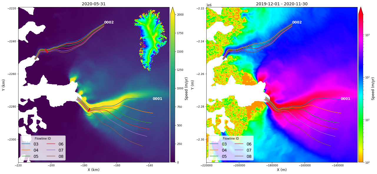
    time2        datetime64[ns] 2020-11-30

xarray.DataArray

'VelocitySeries'

• time: 1
• band: 3
• y: 856
• x: 474

• dask.array<chunksize=(1, 1, 512, 474), meta=np.ndarray>

  Array Chunk Bytes 4.64 MiB 0.93 MiB Shape (1, 3, 856, 474) (1, 1, 512, 474) Count 38 Tasks 6 Chunks Type float32 numpy.ndarray

• Coordinates: (9)
  • band
    (band)
    <U2
    'vx' 'vy' 'vv'

    array(['vx', 'vy', 'vv'], dtype='<U2')

  • x
    (x)
    float64
    -6.575e+05 -6.543e+05 ... 8.563e+05

    array([-657499.78903 , -654299.367089, -651098.945148, ...,  849898.945148,
            853099.367089,  856299.78903 ])

  • y
    (y)
    float64
    -6.407e+05 ... -3.377e+06

    array([ -640700.46729 ,  -643901.401869,  -647102.336449, ..., -3371097.663551,
           -3374298.598131, -3377499.53271 ])

  • spatial_ref
    ()
    int64
    0

    crs_wkt :

    PROJCS["WGS 84 / NSIDC Sea Ice Polar Stereographic North",GEOGCS["WGS 84",DATUM["WGS_1984",SPHEROID["WGS 84",6378137,298.257223563,AUTHORITY["EPSG","7030"]],AUTHORITY["EPSG","6326"]],PRIMEM["Greenwich",0,AUTHORITY["EPSG","8901"]],UNIT["degree",0.0174532925199433,AUTHORITY["EPSG","9122"]],AUTHORITY["EPSG","4326"]],PROJECTION["Polar_Stereographic"],PARAMETER["latitude_of_origin",70],PARAMETER["central_meridian",-45],PARAMETER["false_easting",0],PARAMETER["false_northing",0],UNIT["metre",1,AUTHORITY["EPSG","9001"]],AXIS["Easting",SOUTH],AXIS["Northing",SOUTH],AUTHORITY["EPSG","3413"]]

    semi_major_axis :

    6378137.0

    semi_minor_axis :

    6356752.314245179

    inverse_flattening :

    298.257223563

    reference_ellipsoid_name :

    WGS 84

    longitude_of_prime_meridian :

    0.0

    prime_meridian_name :

    Greenwich

    geographic_crs_name :

    WGS 84

    horizontal_datum_name :

    World Geodetic System 1984

    projected_crs_name :

    WGS 84 / NSIDC Sea Ice Polar Stereographic North

    grid_mapping_name :

    polar_stereographic

    standard_parallel :

    70.0

    straight_vertical_longitude_from_pole :

    -45.0

    false_easting :

    0.0

    false_northing :

    0.0

    spatial_ref :

    PROJCS["WGS 84 / NSIDC Sea Ice Polar Stereographic North",GEOGCS["WGS 84",DATUM["WGS_1984",SPHEROID["WGS 84",6378137,298.257223563,AUTHORITY["EPSG","7030"]],AUTHORITY["EPSG","6326"]],PRIMEM["Greenwich",0,AUTHORITY["EPSG","8901"]],UNIT["degree",0.0174532925199433,AUTHORITY["EPSG","9122"]],AUTHORITY["EPSG","4326"]],PROJECTION["Polar_Stereographic"],PARAMETER["latitude_of_origin",70],PARAMETER["central_meridian",-45],PARAMETER["false_easting",0],PARAMETER["false_northing",0],UNIT["metre",1,AUTHORITY["EPSG","9001"]],AXIS["Easting",SOUTH],AXIS["Northing",SOUTH],AUTHORITY["EPSG","3413"]]

    GeoTransform :

    -659100.0 3200.4219409282696 0.0 -639100.0 0.0 -3200.9345794392525

    array(0)

  • time
    (time)
    datetime64[ns]
    2020-05-31T12:00:00

    array(['2020-05-31T12:00:00.000000000'], dtype='datetime64[ns]')

  • name
    ()
    <U4
    'None'

    array('None', dtype='<U4')

  • _FillValue
    ()
    float64
    -2e+09

    array(-2.e+09)

  • time1
    ()
    datetime64[ns]
    2019-12-01

    array('2019-12-01T00:00:00.000000000', dtype='datetime64[ns]')

  • time2
    ()
    datetime64[ns]
    2020-11-30

    array('2020-11-30T00:00:00.000000000', dtype='datetime64[ns]')

• Attributes: (0)

Display Flowlines and Velocity

In the next cell, we put the above pieces together:

• Display speed with linear and log color bars,

• Use the overview image for an inset.

• Plot the flowline line locations.

• For a later plot, extract a point 10-km along each flowline using myFlowlines[glacierId].extractPoints(10, None, units='km')

# set up figure and axis
#%matplotlib inline
fig, axes = plt.subplots(1, 2, figsize=(21, 12))

# Create a dictionary for accumulating glacier points
glacierPoints = {}
# generate a color dict that spans all flowline ids, using method from a flowline instance
flowlineColors = list(myFlowlines.values())[0].genColorDict(flowlineIDs=flowlineIDs)
# Plot velocity maps
# Saturate at 2000 m/yr to preserve slow detail
myVelSeries.displayVelForDate('2020-01-01', ax=axes[0], labelFontSize=12, plotFontSize=9, titleFontSize=14, 
                              vmin=0, vmax=2000, units='km', scale='linear', colorBarSize='3%') 
myVelSeries.displayVelForDate('2020-01-01', ax=axes[1], labelFontSize=12, plotFontSize=9, titleFontSize=14, 
                              vmin=1, vmax=3000, units='m', scale='log', midDate=False, colorBarSize='3%')
# Plot location inset
height = 3
axInset = inset_axes(axes[0], width=height * myOverview.sx/myOverview.sy, height=height, loc=1)
myOverview.displayVelForDate(None, ax=axInset, vmin=1, vmax=3000, colorBar=False, scale='log', title='')
axInset.plot(*myVelSeries.outline(), color='r')
axInset.axis('off')
#
# Loop over each glacier and plot the flowlines
for glacierId in myFlowlines:
    # Plot the flowline Match units to the map
    myFlowlines[glacierId].plotFlowlineLocations(ax=axes[0], units='km', colorDict=flowlineColors)
    myFlowlines[glacierId].plotFlowlineLocations(ax=axes[1], units='m', colorDict=flowlineColors)
    # 
    myFlowlines[glacierId].plotGlacierName(ax=axes[0], units='km', color='w', fontsize=12,fontweight='bold', first=False)
    myFlowlines[glacierId].plotGlacierName(ax=axes[1], units='m', color='w', fontsize=12,fontweight='bold', first=False)
    # Generates points 10km from downstream end of each flowline
    points10km = myFlowlines[glacierId].extractPoints(10, None, units='km')
    glacierPoints[glacierId] = points10km
    for key in points10km:
        axes[0].plot(*points10km[key], 'r.')
#
# Add legend
for ax in axes:
    # Create a dict of unique labels for legend
    h, l = ax.get_legend_handles_labels()
    by_label = dict(zip(l, h)) # will overwrite identical entries to produce unique values
    ax.legend(by_label.values(), by_label.keys(), title='Flowline ID', ncol=2, loc='lower left', fontsize=14)
#fig.tight_layout()

Interpolation

A common function with the velocity date is interpolating data for plotting points or profiles, which can be easily done with the nisarVelSeries.interp method.

# Using km
vx, vy, vv = myVelSeries.interp(*myFlowlines[glacierId].xykm(), units='km')
print(vx.shape, vx[0, 100], vy[0, 100], vv[0, 100])

# or units of meters
vx, vy, vv = myVelSeries.interp(*myFlowlines[glacierId].xym(), units='m')
print(vx.shape, vx[0, 100], vy[0, 100], vv[0, 100])
# or entirely different coordinate system
xytoll = pyproj.Transformer.from_crs(3413, 4326)
lat, lon = xytoll.transform(*myFlowlines[glacierId].xym())
vx, vy, vv = myVelSeries.interp(lat, lon, sourceEPSG=4326)
print(vx.shape, vx[0, 100], vy[0, 100], vv[0, 100])
# Or would prefer an xarray rather than nparray
result = myVelSeries.interp(*myFlowlines[glacierId].xykm(), units='km', returnXR=True)
result

(6, 181) -77.83922891005291 -11.383531758615678 78.66828524051097
(6, 181) -77.83922891005291 -11.383531758615678 78.66828524051097
(6, 181) -77.83922891003112 -11.383531758575606 78.66828524048344

<xarray.DataArray 'VelocitySeries' (band: 3, time: 6, dim_0: 181)>
array([[[          nan,           nan,   -9.12698043, ...,
         -100.56018746, -100.4755341 , -100.34382731],
        [          nan,           nan,           nan, ...,
          -99.63389458,  -99.29062583,  -98.89326907],
        [          nan,           nan,           nan, ...,
         -100.97662177,  -99.90459653,  -99.93636591],
        [          nan,           nan,           nan, ...,
         -105.82850221, -105.12042442, -104.68619218],
        [          nan,           nan,           nan, ...,
         -101.25187846, -100.63794841, -100.33250194],
        [          nan,           nan,           nan, ...,
          -99.99893708,  -99.24659621,  -98.67511691]],

       [[          nan,           nan, -172.07627342, ...,
          -69.70465312,  -67.66019117,  -67.45838283],
        [          nan,           nan,           nan, ...,
          -70.35840163,  -70.69637773,  -71.8085976 ],
        [          nan,           nan,           nan, ...,
          -60.65890769,  -61.40574   ,  -63.7975528 ],
        [          nan,           nan,           nan, ...,
          -64.53959303,  -65.29289975,  -66.84651283],
        [          nan,           nan,           nan, ...,
          -61.57684518,  -62.93505144,  -66.51665249],
        [          nan,           nan,           nan, ...,
          -62.08597838,  -61.9260305 ,  -63.827031  ]],

       [[          nan,           nan,  172.32232531, ...,
          122.357786  ,  121.14074063,  120.91350398],
        [          nan,           nan,           nan, ...,
          121.97283295,  121.88811503,  122.21810542],
        [          nan,           nan,           nan, ...,
          117.79736177,  117.27126169,  118.56589702],
        [          nan,           nan,           nan, ...,
          123.95721595,  123.74802047,  124.21122317],
        [          nan,           nan,           nan, ...,
          118.50652274,  118.70036278,  120.38466664],
        [          nan,           nan,           nan, ...,
          117.70631124,  116.98390201,  117.52199928]]])
Coordinates:
  * band         (band) <U2 'vx' 'vy' 'vv'
  * time         (time) datetime64[ns] 2015-06-01 ... 2020-05-31T12:00:00
    name         <U4 'None'
    _FillValue   float64 -2e+09
    time1        (time) datetime64[ns] 2014-12-01 2015-12-01 ... 2019-12-01
    time2        (time) datetime64[ns] 2015-11-30 2016-11-30 ... 2020-11-30
    spatial_ref  int64 0
    x            (dim_0) float64 -2.1e+05 -2.098e+05 ... -1.679e+05 -1.676e+05
    y            (dim_0) float64 -2.251e+06 -2.25e+06 ... -2.229e+06 -2.229e+06
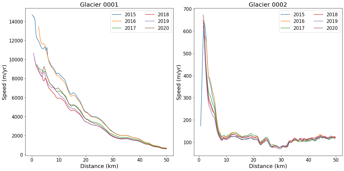
Dimensions without coordinates: dim_0

xarray.DataArray

'VelocitySeries'

• band: 3
• time: 6
• dim_0: 181

• nan nan -9.127 -37.83 -106.1 -171.0 ... 122.6 120.6 117.7 117.0 117.5

  array([[[          nan,           nan,   -9.12698043, ...,
           -100.56018746, -100.4755341 , -100.34382731],
          [          nan,           nan,           nan, ...,
            -99.63389458,  -99.29062583,  -98.89326907],
          [          nan,           nan,           nan, ...,
           -100.97662177,  -99.90459653,  -99.93636591],
          [          nan,           nan,           nan, ...,
           -105.82850221, -105.12042442, -104.68619218],
          [          nan,           nan,           nan, ...,
           -101.25187846, -100.63794841, -100.33250194],
          [          nan,           nan,           nan, ...,
            -99.99893708,  -99.24659621,  -98.67511691]],
  
         [[          nan,           nan, -172.07627342, ...,
            -69.70465312,  -67.66019117,  -67.45838283],
          [          nan,           nan,           nan, ...,
            -70.35840163,  -70.69637773,  -71.8085976 ],
          [          nan,           nan,           nan, ...,
            -60.65890769,  -61.40574   ,  -63.7975528 ],
          [          nan,           nan,           nan, ...,
            -64.53959303,  -65.29289975,  -66.84651283],
          [          nan,           nan,           nan, ...,
            -61.57684518,  -62.93505144,  -66.51665249],
          [          nan,           nan,           nan, ...,
            -62.08597838,  -61.9260305 ,  -63.827031  ]],
  
         [[          nan,           nan,  172.32232531, ...,
            122.357786  ,  121.14074063,  120.91350398],
          [          nan,           nan,           nan, ...,
            121.97283295,  121.88811503,  122.21810542],
          [          nan,           nan,           nan, ...,
            117.79736177,  117.27126169,  118.56589702],
          [          nan,           nan,           nan, ...,
            123.95721595,  123.74802047,  124.21122317],
          [          nan,           nan,           nan, ...,
            118.50652274,  118.70036278,  120.38466664],
          [          nan,           nan,           nan, ...,
            117.70631124,  116.98390201,  117.52199928]]])

• Coordinates: (9)
  • band
    (band)
    <U2
    'vx' 'vy' 'vv'

    array(['vx', 'vy', 'vv'], dtype='<U2')

  • time
    (time)
    datetime64[ns]
    2015-06-01 ... 2020-05-31T12:00:00

    array(['2015-06-01T00:00:00.000000000', '2016-05-31T12:00:00.000000000',
           '2017-06-01T00:00:00.000000000', '2018-06-01T00:00:00.000000000',
           '2019-06-01T00:00:00.000000000', '2020-05-31T12:00:00.000000000'],
          dtype='datetime64[ns]')

  • name
    ()
    <U4
    'None'

    array('None', dtype='<U4')

  • _FillValue
    ()
    float64
    -2e+09

    array(-2.e+09)

  • time1
    (time)
    datetime64[ns]
    2014-12-01 ... 2019-12-01

    array(['2014-12-01T00:00:00.000000000', '2015-12-01T00:00:00.000000000',
           '2016-12-01T00:00:00.000000000', '2017-12-01T00:00:00.000000000',
           '2018-12-01T00:00:00.000000000', '2019-12-01T00:00:00.000000000'],
          dtype='datetime64[ns]')

  • time2
    (time)
    datetime64[ns]
    2015-11-30 ... 2020-11-30

    array(['2015-11-30T00:00:00.000000000', '2016-11-30T00:00:00.000000000',
           '2017-11-30T00:00:00.000000000', '2018-11-30T00:00:00.000000000',
           '2019-11-30T00:00:00.000000000', '2020-11-30T00:00:00.000000000'],
          dtype='datetime64[ns]')

  • spatial_ref
    ()
    int64
    0

    crs_wkt :

    PROJCS["WGS 84 / NSIDC Sea Ice Polar Stereographic North",GEOGCS["WGS 84",DATUM["WGS_1984",SPHEROID["WGS 84",6378137,298.257223563,AUTHORITY["EPSG","7030"]],AUTHORITY["EPSG","6326"]],PRIMEM["Greenwich",0,AUTHORITY["EPSG","8901"]],UNIT["degree",0.0174532925199433,AUTHORITY["EPSG","9122"]],AUTHORITY["EPSG","4326"]],PROJECTION["Polar_Stereographic"],PARAMETER["latitude_of_origin",70],PARAMETER["central_meridian",-45],PARAMETER["false_easting",0],PARAMETER["false_northing",0],UNIT["metre",1,AUTHORITY["EPSG","9001"]],AXIS["Easting",SOUTH],AXIS["Northing",SOUTH],AUTHORITY["EPSG","3413"]]

    semi_major_axis :

    6378137.0

    semi_minor_axis :

    6356752.314245179

    inverse_flattening :

    298.257223563

    reference_ellipsoid_name :

    WGS 84

    longitude_of_prime_meridian :

    0.0

    prime_meridian_name :

    Greenwich

    geographic_crs_name :

    WGS 84

    horizontal_datum_name :

    World Geodetic System 1984

    projected_crs_name :

    WGS 84 / NSIDC Sea Ice Polar Stereographic North

    grid_mapping_name :

    polar_stereographic

    standard_parallel :

    70.0

    straight_vertical_longitude_from_pole :

    -45.0

    false_easting :

    0.0

    false_northing :

    0.0

    spatial_ref :

    PROJCS["WGS 84 / NSIDC Sea Ice Polar Stereographic North",GEOGCS["WGS 84",DATUM["WGS_1984",SPHEROID["WGS 84",6378137,298.257223563,AUTHORITY["EPSG","7030"]],AUTHORITY["EPSG","6326"]],PRIMEM["Greenwich",0,AUTHORITY["EPSG","8901"]],UNIT["degree",0.0174532925199433,AUTHORITY["EPSG","9122"]],AUTHORITY["EPSG","4326"]],PROJECTION["Polar_Stereographic"],PARAMETER["latitude_of_origin",70],PARAMETER["central_meridian",-45],PARAMETER["false_easting",0],PARAMETER["false_northing",0],UNIT["metre",1,AUTHORITY["EPSG","9001"]],AXIS["Easting",SOUTH],AXIS["Northing",SOUTH],AUTHORITY["EPSG","3413"]]

    GeoTransform :

    -220100.0 200.0 0.0 -2219100.0 0.0 -200.0

    array(0)

  • x
    (dim_0)
    float64
    -2.1e+05 -2.098e+05 ... -1.676e+05

    array([-210012.643529, -209819.158817, -209641.128082, -209451.254745,
           -209272.491977, -209140.913445, -209023.915017, -208879.596386,
           -208879.596386, -208735.277755, -208580.625158, -208447.839052,
           -208331.350863, -208224.063279, -208123.125088, -208025.601701,
           -207929.63692 , -207831.998867, -207729.131596, -207616.445626,
           -207485.558876, -207328.917491, -207136.650365, -206898.904706,
           -206648.904706, -206398.904706, -206148.904706, -205898.904706,
           -205648.904706, -205398.904706, -205148.904706, -204898.904706,
           -204648.904706, -204398.904706, -204148.904706, -203898.904706,
           -203648.904706, -203398.904706, -203148.904706, -202898.904706,
           -202648.904706, -202398.904706, -202148.904706, -201898.904706,
           -201648.904706, -201398.904706, -201148.904706, -200898.904706,
           -200648.904706, -200398.904706, -200148.904706, -199898.904706,
           -199648.904706, -199398.904706, -199148.904706, -198898.904706,
           -198648.904706, -198398.904706, -198148.904706, -197898.904706,
           -197648.904706, -197398.904706, -197148.904706, -196898.904706,
           -196648.904706, -196398.904706, -196148.904706, -195898.904706,
           -195648.904706, -195398.904706, -195148.904706, -194898.904706,
           -194648.904706, -194398.904706, -194148.904706, -193898.904706,
           -193648.904706, -193398.904706, -193148.904706, -192898.904706,
           -192648.904706, -192398.904706, -192148.904706, -191898.904706,
           -191648.904706, -191398.904706, -191148.904706, -190898.904706,
           -190648.904706, -190398.904706, -190148.904706, -189898.904706,
           -189648.904706, -189398.904706, -189148.904706, -188898.904706,
           -188648.904706, -188398.904706, -188148.904706, -187898.904706,
           -187648.904706, -187398.904706, -187148.904706, -186898.904706,
           -186648.904706, -186398.904706, -186148.904706, -185898.904706,
           -185648.904706, -185398.904706, -185148.904706, -184898.904706,
           -184648.904706, -184398.904706, -184148.904706, -183898.904706,
           -183648.904706, -183398.904706, -183148.904706, -182898.904706,
           -182648.904706, -182398.904706, -182148.904706, -181898.904706,
           -181648.904706, -181398.904706, -181148.904706, -180898.904706,
           -180648.904706, -180398.904706, -180148.904706, -179898.904706,
           -179648.904706, -179398.904706, -179148.904706, -178898.904706,
           -178648.904706, -178398.904706, -178148.904706, -177898.904706,
           -177648.904706, -177398.904706, -177148.904706, -176898.904706,
           -176648.904706, -176398.904706, -176148.904706, -175898.904706,
           -175648.904706, -175398.904706, -175148.904706, -174898.904706,
           -174648.904706, -174398.904706, -174148.904706, -173898.904706,
           -173648.904706, -173398.904706, -173148.904706, -172898.904706,
           -172648.904706, -172398.904706, -172148.904706, -171898.904706,
           -171648.904706, -171398.904706, -171148.904706, -170898.904706,
           -170648.904706, -170398.904706, -170148.904706, -169898.904706,
           -169648.904706, -169398.904706, -169148.904706, -168898.904706,
           -168648.904706, -168398.904706, -168148.904706, -167898.904706,
           -167648.904706])

  • y
    (dim_0)
    float64
    -2.251e+06 -2.25e+06 ... -2.229e+06

    array([-2250687.500532, -2250437.500532, -2250187.500532, -2249937.500532,
           -2249687.500532, -2249437.500532, -2249187.500532, -2248937.500532,
           -2248937.500532, -2248687.500532, -2248437.500532, -2248187.500532,
           -2247937.500532, -2247687.500532, -2247437.500532, -2247187.500532,
           -2246937.500532, -2246687.500532, -2246437.500532, -2246187.500532,
           -2245937.500532, -2245687.500532, -2245437.500532, -2245187.500532,
           -2245000.245072, -2244877.724702, -2244802.800592, -2244765.132125,
           -2244754.08338 , -2244759.595896, -2244775.812244, -2244800.002143,
           -2244827.934032, -2244854.918411, -2244879.126426, -2244901.211886,
           -2244921.580466, -2244939.07737 , -2244951.80443 , -2244958.306895,
           -2244957.036195, -2244946.372941, -2244925.99873 , -2244895.978208,
           -2244856.045478, -2244805.884753, -2244745.524676, -2244675.113281,
           -2244596.172494, -2244509.156784, -2244414.208809, -2244313.577133,
           -2244208.518144, -2244102.153883, -2243997.153915, -2243894.201986,
           -2243795.644302, -2243705.756319, -2243628.689468, -2243566.375675,
           -2243517.846044, -2243479.006996, -2243442.461316, -2243401.428191,
           -2243351.448235, -2243289.195143, -2243212.62758 , -2243122.374351,
           -2243022.747103, -2242918.537949, -2242813.754613, -2242709.435094,
           -2242606.937299, -2242508.483562, -2242415.387085, -2242326.738441,
           -2242241.96128 , -2242159.57985 , -2242075.598726, -2241985.155824,
           -2241882.822641, -2241768.301348, -2241644.883568, -2241523.753081,
           -2241412.045541, -2241311.151388, -2241218.385957, -2241131.867049,
           -2241052.313204, -2240982.120649, -2240922.590489, -2240871.143364,
           -2240823.296594, -2240776.271034, -2240731.234944, -2240692.116247,
           -2240660.329541, -2240635.319836, -2240616.01236 , -2240600.079476,
           -2240584.040528, -2240562.86629 , -2240532.384663, -2240491.079091,
           -2240442.261622, -2240390.486424, -2240334.737622, -2240274.835751,
           -2240214.847478, -2240156.559666, -2240095.340187, -2240027.272639,
           -2239952.399614, -2239872.144769, -2239784.36888 , -2239688.751836,
           -2239582.856609, -2239468.583477, -2239356.718905, -2239249.856794,
           -2239144.536355, -2239037.099176, -2238920.43824 , -2238790.856888,
           -2238646.021301, -2238489.767418, -2238340.363877, -2238206.292455,
           -2238077.062293, -2237939.685224, -2237787.278745, -2237616.430054,
           -2237436.614799, -2237255.558181, -2237073.804709, -2236891.432466,
           -2236700.672208, -2236500.622086, -2236297.485868, -2236087.714404,
           -2235871.328427, -2235645.881954, -2235422.825758, -2235216.769283,
           -2235022.170055, -2234820.575992, -2234609.030752, -2234389.86845 ,
           -2234178.888421, -2233981.126555, -2233788.966079, -2233605.141782,
           -2233433.027961, -2233269.712677, -2233114.639245, -2232959.866468,
           -2232800.25541 , -2232635.203707, -2232470.989524, -2232311.663792,
           -2232147.405213, -2231982.559273, -2231824.759703, -2231672.351323,
           -2231523.36246 , -2231374.028822, -2231227.005184, -2231084.113462,
           -2230943.922942, -2230802.823846, -2230659.681837, -2230512.987011,
           -2230360.044896, -2230205.528344, -2230052.639186, -2229895.360793,
           -2229739.576395, -2229589.597666, -2229443.151603, -2229293.542494,
           -2229138.649249])

• Attributes: (0)

Plot Central Flowlines at Different Times

This example will demonstrate plotting the nominally central flowline (‘06’) for each of the six years for which there are currently data. While we are using flow lines here, any profile data could be used (e.g., a flux gate).

flowlineId ='06'  # Flowline id to plot
fig, axes = plt.subplots(np.ceil(len(myFlowlines)/4).astype(int), 2, figsize=(16, 8))  # Setup plot
# Loop over glaciers
for glacierId, ax in zip(myFlowlines, axes.flatten()):
    #
    # return interpolated values as vx(time index, distance index)
    vx, vy, vv = myVelSeries.interp(*myFlowlines[glacierId].xykm(), units='km')
    #
    # loop over each profile by time
    for speed, myDate in zip(vv, myVelSeries.time):
        ax.plot(myFlowlines[glacierId].distancekm(), speed, label=myDate.year)
    #
    # pretty up plot
    ax.legend(ncol=2, loc='upper right', fontsize=15)
    ax.set_xlabel('Distance (km)', fontsize=18)
    ax.set_ylabel('Speed (m/yr)', fontsize=18)
    ax.set_title(f'Glacier {glacierId}', fontsize=20)
#
# Resize tick labels 
for ax in axes.flatten():
    ax.tick_params(axis='both', labelsize=15)
plt.tight_layout()

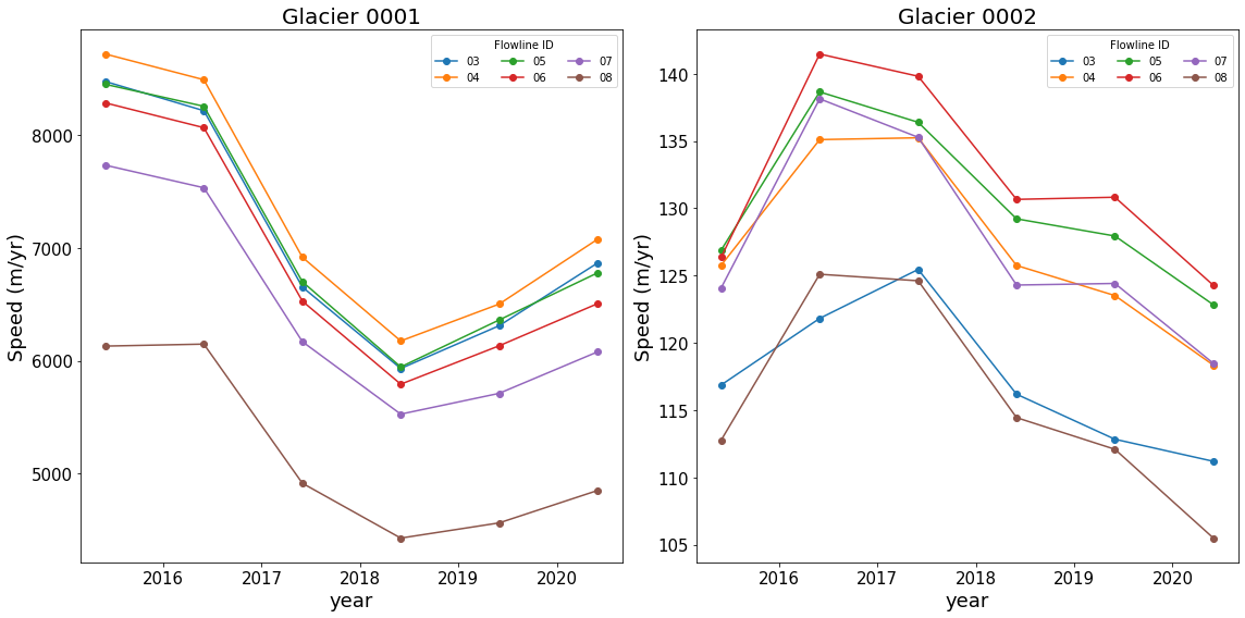
Plot Points Through Time

When the map plots were generated above, a set of points 10-k from the start of each flowline was extracted:

glacierPoints

{'0001': {'03': (-176.56832111994873, -2281.0994802378723),
  '04': (-176.57938979911765, -2281.5335680932617),
  '05': (-176.57002817972838, -2281.9249696551415),
  '06': (-176.79220987043246, -2282.204119702424),
  '07': (-176.9666900075591, -2282.481895335485),
  '08': (-177.43129335281543, -2282.7171334333398)},
 '0002': {'03': (-203.39890470601097, -2244.9390773695413),
  '04': (-203.05275750822682, -2245.3549816898053),
  '05': (-203.02191562572793, -2245.7134285462275),
  '06': (-202.7513660612219, -2246.0637465671216),
  '07': (-202.46742712091572, -2246.4450735405717),
  '08': (-202.14758624325026, -2246.820176873798)}}

The time series for each set of. points can be plotted as:

#%matplotlib inline
fig, axes = plt.subplots(1, 2, figsize=(16, 8))
# Loop over glaciers
for glacierId, ax in zip(glacierPoints, axes.flatten()):
    # Loop over flowlines
    for flowlineId in glacierPoints[glacierId]:
        #
        # interpolate to get results vx(time index) for each point
        vx, vy, v = myVelSeries.interp(*glacierPoints[glacierId][flowlineId], units='km')
        ax.plot(myVelSeries.time, v, marker='o',  linestyle='-', color=flowlineColors[flowlineId],label=f'{flowlineId}')
    #
    # pretty up plot
    ax.legend(ncol=3, loc='upper right', title='Flowline ID')
    ax.set_xlabel('year', fontsize=18)
    ax.set_ylabel('Speed (m/yr)', fontsize=18)
    ax.set_title(f'Glacier {glacierId}', fontsize=20)
#
# Resize tick labels 
for ax in axes.flatten():
    ax.tick_params(axis='both', labelsize=15)
plt.tight_layout()

Save the Data

While it is convenient to work the date remotely, its nice to be be able to save the data for further processing.

The downloaded subset can be saved in a netcdf and reloaded for to velSeries instance for later analysis.

Note makes sure the data have been subsetted so only the the subset will be saved (~15MB in this example). If not, the entire Greeland data set will be saved (370GB).

Change saveData and reloadData below to test this capability.

saveData = True # Set to True to save data
if saveData:
    myVelSeries.toNetCDF('Glaciers1-2example.nc')

Now open open the file and redo a plot from above with the saved data.

reloadData = True  # Set to True to reload the saved data
if reloadData:
    fig, axes = plt.subplots(np.ceil(len(myFlowlines)/2).astype(int), 2, figsize=(16, 8))  # Setup plot
    myVelCDF = nisar.nisarVelSeries() # Create Series
    myVelCDF.readSeriesFromNetCDF('Glaciers1-2example.nc')
    #
    for glacierId, ax in zip(myFlowlines, axes.flatten()):
        # return interpolated values as vx(time index, distance index)
        vx, vy, vv = myVelCDF.interp(*myFlowlines[glacierId].xykm(), units='km')
        # loop over each profile by time
        for speed, myDate in zip(vv, myVelSeries.time):
            ax.plot(myFlowlines[glacierId].distancekm(), speed, label=myDate.year)
        # pretty up plot
        ax.legend(ncol=2, loc='upper right', fontsize=15)
        ax.set_xlabel('Distance (km)', fontsize=18)
        ax.set_ylabel('Speed (m/yr)', fontsize=18)
        ax.set_title(f'Glacier {glacierId}', fontsize=20)
# For other combinations could have 
    for ax in axes.flatten():
        ax.tick_params(axis='both', labelsize=15)
    plt.tight_layout()

Summary for GrIMP Data

Using the nisardev and grimp we were easily able to perform many of the typical functions needed for the analysis of glaciers by accesssing remote GrIMP data such as:

• Accessing stacks of velocity data;

• Display velocity maps; and

• Interpolating data to points or lines;

When working with larger data sets (e.g., the 300+ 6/12 day velocity maps at NSIDC), downloads can take longer (several minutes), but are still 2 to 3 orders of magnitude faster than downloading the full data set.

Once downloaded, the data are easily saved for later use.

Other notebooks demonstrated the use of these tools are available through GrIMPNotebooks repo at github.

As mentioned above, velocity data can help provide context for elevation change measurements. Next we look at elevation change for the Jakobshavn region.

Comparing ICESat-2 Data with Other Datasets

Last time, we did a bit of work to add ICESat-2 and Operation Icebridge data to Pandas Dataframes. We only covered the basic operations that you can do with Pandas, so today we are going to do a more thorough analysis of the data here.

Since we already downloaded the ICESat-2/ATM files of interest, we are not going to use icepyx just yet - we will go ahead and reload the data from yesterday.

(Prompt) I forgot how to load the ICESat-2 data from a .h5 file. What do I need to do?

(Prompt) I also forgot how to load the ATM data. How do I read the CSV?

We established last time that ATM aligns best with the central ICESat-2 beams, particularly the central strong beam (GT2L). Let’s see if that is reflected in the elevation profiles…

# Load the ICESat-2 data
is2_file = 'processed_ATL06_20190420093051_03380303_005_01_full.h5'
with h5py.File(is2_file, 'r') as f:
    is2_gt2r = pd.DataFrame(data={'lat': f['gt2r/land_ice_segments/latitude'][:],
                                  'lon': f['gt2r/land_ice_segments/longitude'][:],
                                  'elev': f['gt2r/land_ice_segments/h_li'][:]}) # Central weak beam
    is2_gt2l = pd.DataFrame(data={'lat': f['gt2l/land_ice_segments/latitude'][:],
                                  'lon': f['gt2l/land_ice_segments/longitude'][:],
                                  'elev': f['gt2l/land_ice_segments/h_li'][:]}) # Central strong beam
    
# Load the ATM data
atm_file = 'ILATM2_20190506_151600_smooth_nadir3seg_50pt.csv'
atm_l2 = pd.read_csv(atm_file)

# Look only at the nadir track
atm_l2 = atm_l2[atm_l2['Track_Identifier']==0]

# Change the longitudes to be consistent with ICESat-2
atm_l2['Longitude(deg)'] -= 360

# Subset the ICESat-2 data to the ATM latitudes
is2_gt2r = is2_gt2r[(is2_gt2r['lat']<atm_l2['Latitude(deg)'].max()) & (is2_gt2r['lat']>atm_l2['Latitude(deg)'].min())]
is2_gt2l = is2_gt2l[(is2_gt2l['lat']<atm_l2['Latitude(deg)'].max()) & (is2_gt2l['lat']>atm_l2['Latitude(deg)'].min())]

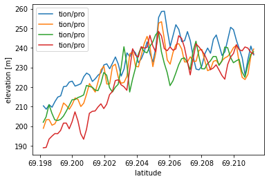
# Make a 2D plot of along-track surface height
import matplotlib.pyplot as plt

#%matplotlib widget
fig, ax = plt.subplots(1, 1)
plt.plot(is2_gt2r['lat'], is2_gt2r['elev'], label='gt2r')
plt.plot(is2_gt2l['lat'], is2_gt2l['elev'], label='gt2l')
plt.plot(atm_l2['Latitude(deg)'], atm_l2['WGS84_Ellipsoid_Height(m)'], label='atm')
plt.xlabel('latitude')
plt.ylabel('elevation [m]')
plt.xlim([69.185, 69.275])
plt.ylim([100, 550])
plt.legend()
plt.show()

Sure enough, GT2L and ATM match very well! Since they are very close to each other, we can do a quick accuracy assessment between the two.

The ATM DataFrame is larger than the ICESat-2 dataframe, so we’re going to apply a simple spline interpolant to downscale the ICESat-2 data.

from scipy.interpolate import splrep,splev
fig, ax = plt.subplots(1, 1)
# Apply a spline interpolant to the ICESat-2 data
spl = splrep(is2_gt2l['lat'], is2_gt2l['elev'], s=0)
is2_spl = splev(atm_l2['Latitude(deg)'], spl, der=0)

# Calculate GT2L bias and add it to the ATM DataFrame
atm_l2['bias'] = atm_l2['WGS84_Ellipsoid_Height(m)'] - is2_spl
# Plot the bias curve
plt.plot(atm_l2['Latitude(deg)'], atm_l2['bias'])
#plt.plot(atm_l2['Latitude(deg)'], atm_l2['WGS84_Ellipsoid_Height(m)'])
#plt.plot(atm_l2['Latitude(deg)'], is2_spl)
plt.xlabel('latitude')
plt.ylabel('bias [m]')
plt.xlim([69.2, 69.26])
plt.ylim([-20, 20])
plt.show()

print('Mean bias: %s m' %(atm_l2['bias'].mean()))

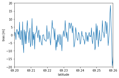
Mean bias: -0.3386212613703729 m

Through some relatively simple operations, we found that ATM and ICESat-2 differ by ~0.33 m on average. Between this plot and the elevation plot above, what do you think might be causing some of the differences?

We will revisit ICESat-2 and ATM near the end of this tutorial. Now, we are going to look at ice velocities and flow lines from the GRIMP project.

Visualization

We are now going to revisit the GRIMP data one last time to visualize all of the data together. We have conducted a bias assessment between the two lidars, so now we are going to look at how the land ice heights change over time.

First let’s take a look at ATM data from previous years. The CSV file we are going to use is pre-processed L2 data for 2011-2018, much like the data from 2019. These flights are slightly east of the 2019 flight, which was adjusted to better align with ICESat-2.

fig, axes = plt.subplots(1, 3, figsize=(15, 5))
# Read in the ATM CSV file
atm_2011_2018 = pd.read_csv('ILATM2_2011_2019_v3.csv')
lltoxy = pyproj.Transformer.from_crs(4326, 3413)

#%matplotlib widget
# Loop through the valid years and plot surface height
years = ['2011', '2013', '2014', '2015', '2016', '2018']
for i,year in enumerate(years):
    lat = atm_2011_2018['Latitude_'+year]
    elev = atm_2011_2018['elev_'+year]
    axes[1].plot(lat, elev, label=year)
#
#
myVelSeries.displayVelForDate('2020-01-01', ax=axes[0], labelFontSize=12, plotFontSize=9, titleFontSize=14, 
                              vmin=1, vmax=3000, units='m', scale='log', midDate=False, colorBarSize='3%', colorBarPosition='bottom')
axes[0].axis('off')
lltoxy = pyproj.Transformer.from_crs(4326, 3413)
for i, year in enumerate(years[3:]):
    lat, lon = atm_2011_2018['Latitude_'+year], atm_2011_2018['Longitude_'+year]
    x, y = lltoxy.transform(lat, lon)
    axes[0].plot(x, y, 'w', linewidth=2)
    v =  myVelSeries.interp(lat, lon, sourceEPSG=4326, returnXR=True).sel(time=datetime.datetime(int(year), 6, 1), 
                                                                          method='nearest').sel(band='vv')
    axes[2].plot(lat, v, label=year)
#
axes[1].set_xlabel('latitude')
axes[1].set_ylabel('elevation [m]')
axes[1].legend()
axes[2].set_xlabel('latitude')
axes[2].set_ylabel('Speed [m/yr]')
axes[2].legend()
fig.tight_layout()

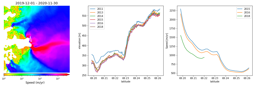
Across these three figures, we can compare the ATM surface heights with ice velocities over the region. It’s obvious that the greatest ice velocities are at the lower elevations, and vice-versa.

We can also see a distinct decrease in ice velocity for 2018 - let’s make a time series to see the ice height changes observed by ATM…

# Set the latitude bounds of the surface trough
lat_bounds = [69.1982, 69.2113]

# 2013 has the longest streak of data over this region. We are going to downscale the other years to its length.
lat_2013 = atm_2011_2018['Latitude_2013'][(atm_2011_2018['Latitude_2013']>lat_bounds[0]) & (atm_2011_2018['Latitude_2013']<lat_bounds[1])]

# First, downscale the 2011 data to 2013 resolution
lat = atm_2011_2018['Latitude_2011']
elev = atm_2011_2018['elev_2011'][(lat>lat_bounds[0]) & (lat<lat_bounds[1])].reset_index(drop=True)
        
lat = lat[(lat>lat_bounds[0]) & (lat<lat_bounds[1])].reset_index(drop=True)
spl = splrep(lat[::-1], elev[::-1], s=0)
slp_2011 = splev(lat_2013, spl, der=0)

# Calculate ice loss relative to 2011
delta_h = [0]
std_h = [0]
for i,year in enumerate(years[1:]): # Start loop at 2013 (2012 has no data)
    if year != 2013: # Downscale other years to 2013 resolution
        lat = atm_2011_2018['Latitude_'+year]
        elev = atm_2011_2018['elev_'+year][(lat>lat_bounds[0]) & (lat<lat_bounds[1])].reset_index(drop=True)
        
        # Downscale the data with splines
        lat = lat[(lat>lat_bounds[0]) & (lat<lat_bounds[1])].reset_index(drop=True)
        spl = splrep(lat[::-1], elev[::-1], s=0)
        spl_year = splev(lat_2013, spl, der=0)
        
        # Now calculate the difference relative to 2011
        delta_h.append((spl_year - slp_2011).mean())
        std_h.append((spl_year - slp_2011).std())
    else:
        lat = atm_2011_2018['Latitude_'+year]
        elev = atm_2011_2018['elev_'+year][(lat>lat_bounds[0]) & (lat<lat_bounds[1])].reset_index(drop=True)
        
        # Calculate the difference relative to 2011
        delta_h.append((elev[::-1] - slp_2011).mean())
        std_h.append((spl_year - slp_2011).std())
    
#%matplotlib widget
fig, ax = plt.subplots(1, 1)
plt.errorbar(years, delta_h, yerr=std_h, marker='.', markersize=12, capsize=4)
plt.xlabel('year')
plt.ylabel('$\Delta$ h [m]')
plt.show()

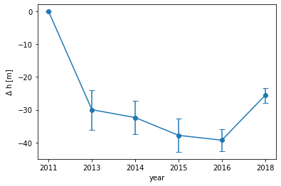
Ta-da!! Using a few operations, we were able to use ATM data to derive a rough time series of ice sheet elevation change over Jakobshavan. We can see that there is a significant loss in ice between 2011 and 2013, followed by a gradual decrease up through 2016. Interestingly, there is a non-negligible increase in ice height in 2018, which may explain the decrease in ice velocity for the same year.

We’re going to try and do the same thing, but for ICESat-2. Because it was launched in late-2018, we are going to try and grab interseasonal measurements from RGT 338 for 2019-2021.

# Time to go through the icepyx routine again!
import icepyx as ipx

# Specifying the necessary icepyx parameters
short_name = 'ATL06'
lat_bounds = [69.1982, 69.2113]
spatial_extent = [-50, 69.1982, -48.5, 69.2113] # KML polygon centered on Jakobshavan
date_range = ['2019-04-01', '2021-12-30']
rgts = ['338'] # IS-2 RGT of interest

# Setup the Query object
region = ipx.Query(short_name, spatial_extent, date_range, tracks=rgts)

# Show the available granules
region.avail_granules(ids=True)

[['ATL06_20190420093051_03380303_005_01.h5',
  'ATL06_20190720051023_03380403_005_01.h5',
  'ATL06_20191019005025_03380503_005_01.h5',
  'ATL06_20200117203009_03380603_005_01.h5',
  'ATL06_20200417160957_03380703_005_01.h5',
  'ATL06_20200717114945_03380803_005_01.h5',
  'ATL06_20201016072931_03380903_005_01.h5',
  'ATL06_20210115030926_03381003_005_01.h5',
  'ATL06_20210415224917_03381103_005_01.h5',
  'ATL06_20210715182907_03381203_005_01.h5',
  'ATL06_20211014140906_03381303_005_01.h5']]

# Set Earthdata credentials
uid = 'uwhackweek'
email = 'hackweekadmin@gmail.com'
region.earthdata_login(uid, email)

# Order the granules
region.order_granules()

Total number of data order requests is  1  for  11  granules.
Data request  1  of  1  is submitting to NSIDC

order ID:  5000003039889
Initial status of your order request at NSIDC is:  processing
Your order status is still  processing  at NSIDC. Please continue waiting... this may take a few moments.

Your order is: complete
NSIDC returned these messages
['Granule 228809321 contained no data within the spatial and/or temporal '
 'subset constraints to be processed',
 'Granule 228960877 contained no data within the spatial and/or temporal '
 'subset constraints to be processed']

path = '/tmp/DataIntegration/'
region.download_granules(path)

Beginning download of zipped output...

Data request 5000003039889 of  1  order(s) is downloaded.
Download complete

import h5py

fig, ax = plt.subplots(1, 1)

# Iterate through the files to grab elevation, and derive elevation differences relative to April 2019
files = ['/tmp/DataIntegration/processed_' + granule for granule in region.avail_granules(ids=True)[0]]

# Get the initial data from April 2019
with h5py.File(files[0]) as f:
    elev_42019 = f['gt2l/land_ice_segments/h_li'][:]
    lat_42019 = f['gt2l/land_ice_segments/latitude'][:]
    plt.plot(lat_42019, elev_42019, label=files[0][16:24])

delta_h = [0]
std_h = [0]
for file in files[1:]:
    try:
        with h5py.File(file) as f:
            cloud_flag = np.mean(f['gt2l/land_ice_segments/geophysical/cloud_flg_asr'][:])
            # Filter out cloudy scenes
            if cloud_flag < 2:
                lat = f['gt2l/land_ice_segments/latitude'][:]
                elev = f['gt2l/land_ice_segments/h_li'][:]
                date = file[16:24] # Get date of IS-2 overpass
                
                # Find the difference relative to April 2019
                delta_h.append(np.mean(elev - elev_42019))
                std_h.append(np.std(elev - elev_42019))
                
                # Plot the elevation data
                plt.plot(lat, elev, label=date)
            else:
                print('Cloudy scene - no data loaded')
    except:
            print('Cloudy scene - no data loaded')
            
plt.xlabel('latitude')
plt.ylabel('elevation [m]')
plt.legend()
plt.show()

Cloudy scene - no data loaded
Cloudy scene - no data loaded
Cloudy scene - no data loaded
Cloudy scene - no data loaded
Cloudy scene - no data loaded
Cloudy scene - no data loaded
Cloudy scene - no data loaded

# Plot the ice sheet change time series
dates = ['20190420','20200117', '20200717', '202110115']
fig, ax = plt.subplots(1, 1)
plt.errorbar(dates, delta_h, yerr=std_h, marker='.', markersize=12, capsize=4)
plt.xlabel('date')
plt.ylabel('$\Delta$ h [m]')
plt.show()

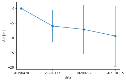
There we go! We lost some data due to cloud cover, and the mean change has some spread, but the ICESat-2 data continues to show a downward trend that was suggested by ATM. Note that these changes are relative to an ICESat-2 observation - if we plotted these on the previous figure, the trend would be even more pronounced!

Summary

🎉 Congratulations! You’ve completed this tutorial and have learned how to:

• Access and plot glacier velocity using GrIMP data and python packages

• Compared ICESat-2 elevations with ATM elevations, and

• Integrated velocities and elevation changes for Jakobshavn into one plot;

These are advanced methods for integrating, analyzing, and visualizing multiple kinds of data sets with ICESat-2, which can be adopted for other kinds of data and analyses.

previous

Data integration with ICESat-2 - Part I

next

ICESat-2 Applications: GrIMP + SlideRule