ICESat-2 Applications: GrIMP + SlideRule
Contents
ICESat-2 Applications: GrIMP + SlideRule
Instructors: Tyler Sutterley and Ian Joughin
Learning Objectives
Goals
Retrieve image mosaics from NSIDC
Subset and view imagery with GrIMP and NISAR tools
Retrieve customized ICESat-2 data with SlideRule
Sample imagery at ICESat-2 photon locations
Working with GrIMP Image Products
Using nisarImage and nisarImageSeries Classes
The Greenland Ice Mapping Project (GrIMP) generates 6 or 12 day Sentinel-1 image mosaics for the Greenland coastline, extending back through 2015, which are archived at NSIDC under NSIDC-0723.
Collectively these products take up more than 2TB, which is more than most users may want to store locally, especially when interested in only a handful of glaciers.
This notebook reviews how to work with subsets of these products downloaded directly from the NSIDC server using the nisarImageSeries class in the nisardev package. We also take advantage of search tools in the grimpfunc package.
Many of the concepts introduced in the early data integration tutorial (e.g., image stacks, xarray, pandas) are used here, though they are often incorporated into class definitions. For those who are curious, the code can be viewed here.
Python Setup
The following packages are needed to execute this notebook.
import os
import dask
from dask.diagnostics import ProgressBar
import geopandas as gpd
import ipyleaflet
import ipywidgets as widgets
import logging
import panel as pn
pn.extension()
import matplotlib.lines
import matplotlib.colors as colors
import matplotlib.gridspec as gridspec
import matplotlib.pyplot as plt
from mpl_toolkits.axes_grid1.inset_locator import inset_axes
import numpy as np
import shapely.geometry
import warnings
# grimp and nisar functions
import grimpfunc as grimp
import nisardev as nisar
# sliderule functions
import sliderule.icesat2
import sliderule.io
import sliderule.ipysliderule
# register progress bar and set workers
ProgressBar().register()
dask.config.set(num_workers=2)
# turn off warnings for demo
warnings.filterwarnings('ignore')
# High resolution matplotlib figures
#%config InlineBackend.figure_format = 'retina'
#plt.rcParams['figure.dpi'] =100 # default=72
Login to EarthData/NSIDC
Unless the data have already been downloaded, users will need to sign in to NSIDC/EarthData to run the rest of the notebook. If a ~/.netrc exists, it will load credentials from there. If not, it will create or append to one after the login has been processed since it is needed by GDAL (see NSIDCLoginNotebook) for more details on security issues.
# Set path for gdal
#!rm ~/.netrc
env = dict(GDAL_HTTP_COOKIEFILE = os.path.expanduser('~/.grimp_download_cookiejar.txt'),
GDAL_HTTP_COOKIEJAR = os.path.expanduser('~/.grimp_download_cookiejar.txt'))
os.environ.update(env)
# Get login
myLogin = grimp.NASALogin() # If login appears not to work, try rerunning this cell
myLogin.view()
Getting login from ~/.netrc
Already logged in. Proceed.
Bounding Box
The examples in this glacier will focus on Zacharie Isstrom in northern Greenland, which can be defined with the following bounding box.
bbox = {'minx': 440000, 'miny': -1140000, 'maxx': 525000, 'maxy': -1080000}
xbox = np.array([bbox[x] for x in ['minx', 'minx', 'maxx', 'maxx', 'minx']]) * 0.001
ybox = np.array([bbox[y] for y in ['miny', 'maxy', 'maxy', 'miny', 'miny']]) * 0.001
Search for Data
Greenland Mapping Project data can be searched for using instances of the class, cmrUrls, which provides a simple graphical and non-graphical interface to the GMP products.
In this example, the search tool is used with mode='image', which restricts the search to NSIDC-0723 image products.
The date range can restricted with firstDate='YYYY-MM-DD' and lastDate='YYYY-MM-DD'.
The images are distributed as uncalibrated image products or calibrated sigma0 (\(\sigma_o\)) and gamma0 (\(\gamma_o\)) products.
In the next cell, we select the image products, which can be specified as productFilter='image'.
In the following example, these search will be carried out based on the input parameters, but a gui search window will popup, which allows the search parameters to be altered.
Image Data
myImageUrls = grimp.cmrUrls(mode='image') # mode image restricts search to the image products
myImageUrls.initialSearch(firstDate='2020-01-01', lastDate='2020-02-24', productFilter='image')
If the search parameters do not need to be altered, then inserting a semicolon at the end of the line will suppress the output. So the corresponding sigma0 and gamma0 products can searched for as:
mySigma0Urls = grimp.cmrUrls(mode='image') # mode image restricts search to the image products
mySigma0Urls.initialSearch(firstDate='2020-01-01', lastDate='2020-02-24', productFilter='sigma0');
myGamma0Urls = grimp.cmrUrls(mode='image') # mode image restricts search to the image products
myGamma0Urls.initialSearch(firstDate='2020-01-01', lastDate='2020-02-24', productFilter='gamma0');
Loading the data
Now that the data have been located, they can be opened for access. The list of urls is given by myImageUrls.getCogs() to be passed into the readSeriesFromTiff method.
myImageSeries = nisar.nisarImageSeries() # Instantiate the series object
myImageSeries.readSeriesFromTiff(myImageUrls.getCogs()) # Open images with lazy reads
myImageSeries.subset # Display map of data layout - add ; to suppress this output
<xarray.DataArray 'image' (time: 10, band: 1, y: 106440, x: 59040)>
dask.array<concatenate, shape=(10, 1, 106440, 59040), dtype=uint8, chunksize=(1, 1, 512, 512), chunktype=numpy.ndarray>
Coordinates:
* band (band) <U5 'image'
* x (x) float64 -6.26e+05 -6.26e+05 -6.259e+05 ... 8.5e+05 8.5e+05
* y (y) float64 -6.95e+05 -6.95e+05 ... -3.356e+06 -3.356e+06
* time (time) datetime64[ns] 2020-01-01T12:00:00 ... 2020-02-24T12:...
name <U4 'None'
_FillValue int64 0
time1 (time) datetime64[ns] 2019-12-30 2020-01-05 ... 2020-02-22
time2 (time) datetime64[ns] 2020-01-04 2020-01-10 ... 2020-02-27
spatial_ref int64 0At nearly 60GB, and this is only 10 of 300+ products, downloading this full data set would take a substantial amount of time, even over a fast network.
But if we use the bounding box defined above, the data set can be limited to just the region of interest as follows:
myImageSeries.subSetImage(bbox)
myImageSeries.subset
<xarray.DataArray 'ImageSeries' (time: 10, band: 1, y: 2400, x: 3400)>
dask.array<getitem, shape=(10, 1, 2400, 3400), dtype=uint8, chunksize=(1, 1, 512, 512), chunktype=numpy.ndarray>
Coordinates:
* band (band) <U5 'image'
* x (x) float64 4.4e+05 4.4e+05 4.401e+05 ... 5.25e+05 5.25e+05
* y (y) float64 -1.08e+06 -1.08e+06 ... -1.14e+06 -1.14e+06
* time (time) datetime64[ns] 2020-01-01T12:00:00 ... 2020-02-24T12:...
name <U4 'None'
_FillValue int64 0
time1 (time) datetime64[ns] 2019-12-30 2020-01-05 ... 2020-02-22
time2 (time) datetime64[ns] 2020-01-04 2020-01-10 ... 2020-02-27
spatial_ref int64 0Here the volume as been greatly reduced. At this stage, the data are still on the NSIDC server. At this point several actions can be taken (e.g., displaying the data), which will automatically download the data using dask. While this implicit download is convenient, it can add time for multiple operations on the data.
While in principle the data are cached by the OS, they can be flushed from the cache, require re-download.
The volume in this example is not large for most computers, so it makes sense to explicitly download the data with as shown next:
myImageSeries.loadRemote()
The process can now be repeated with the sigma0 and gamma0 products.
myGamma0Series = nisar.nisarImageSeries() # Instantiate the series object
myGamma0Series.readSeriesFromTiff(myGamma0Urls.getCogs()) # Open images with lazy reads
myGamma0Series.subSetImage(bbox) # Clip image area
myGamma0Series.loadRemote() # Download clipped regions
mySigma0Series = nisar.nisarImageSeries() # Instantiate the series object
mySigma0Series.readSeriesFromTiff(mySigma0Urls.getCogs()) # Open images with lazy reads
mySigma0Series.subSetImage(bbox) # Clip image area
mySigma0Series.loadRemote() # Download clipped regions
Overview Images
The code above download a small subset, but in some cases its nice to have an overview of the full data set.
As noted above, a nice feature of COGs is that they include image pyramids.
A reduced resolution data set can be created as:
myOverviewSeries = nisar.nisarImageSeries() # Instantiate the series object
myOverviewSeries.readSeriesFromTiff(myImageUrls.getCogs()[0:2], overviewLevel=4) # Open image 4->800 m res (2^(n+1) * original res) = 32*.25
myOverviewSeries.loadRemote()
Image Types
As noted above, the GMP Sentinel image mosaics are produced as:
image (byte scaled with colortable stretch to enhance contrast),
sigm0 (calibrated radar cross section),
gamma0 (calibrated cross section that reduces topographic effects).
A more detailed description of the characteristics of these products is beyond the scope of this notebooks but can be found in the user guide for NSIDC-0723.
In the next cell, we take advantage of the nisarImageSeries.displayImageForDate() method, which will display the image from the stack that lies closest to the specified date.
The following cell illustrates how each of these products can be displayed for a given date with the overview image used as an inset map.
fig, axes = plt.subplots(1, 3, figsize=(24, 11), dpi=72)
#
# Display each image type
for mySeries, ax in zip([myImageSeries, mySigma0Series, myGamma0Series], axes):
mySeries.displayImageForDate(date='2020-01-01', ax=ax, percentile=99) # Clips to 1% (100-99) and 99 percentile
ax.axis('off')
height = 3
fig.tight_layout()
#
# Add an inset map to the first panel
axInset = inset_axes(axes[0], width=height * myOverviewSeries.sx/myOverviewSeries.sy, height=height, loc=2)
myOverviewSeries.displayImageForDate(date='2020-01-01', ax=axInset, colorBar=False, axisOff=True, units='km', masked=0, cmap=plt.cm.gray.with_extremes(bad=(.4,0.4,.4)), title='')
axInset.plot(xbox, ybox, 'r');
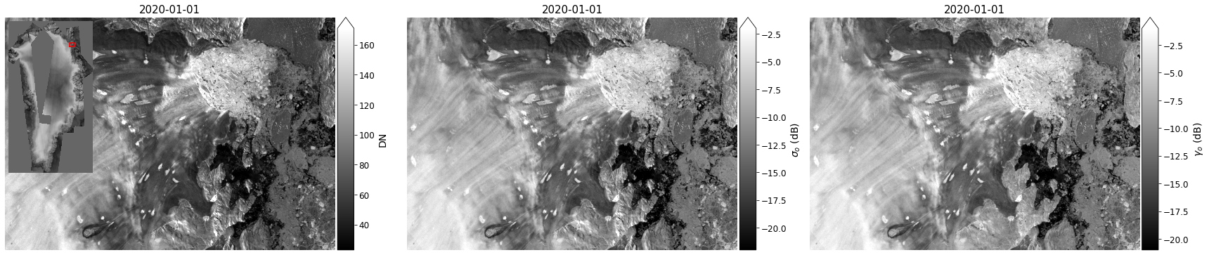
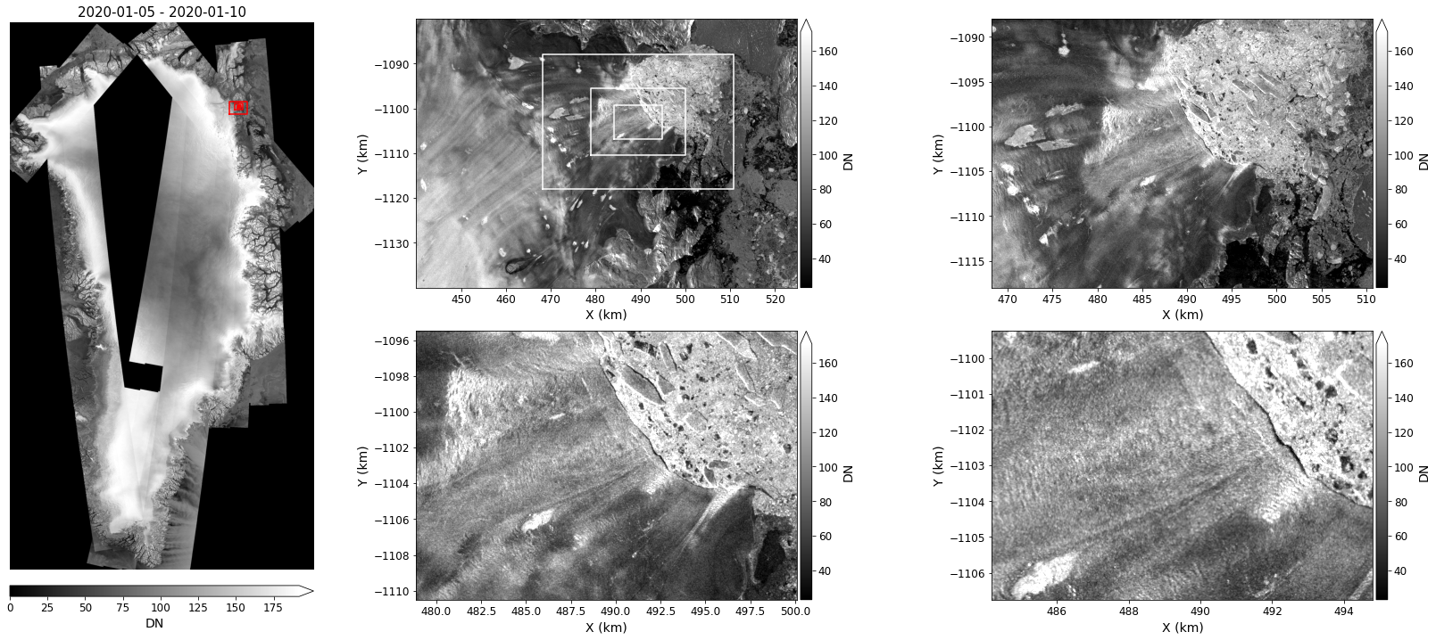
Image Resolution
The figure above does not capture the full resolution of the data.
To better illustrate the 25-m resolution of the data, the following plot zooms in on the center of the image at 4 different levels.
fig = plt.figure(figsize=(23, 10))
#
# Use gridspec to apportion plot area
l, m, n = 4, 7, 7
gs = gridspec.GridSpec(2 * m, l + 2 * n)
#
# Compute center and dimensions of box
xc, yc = (bbox['maxx'] + bbox['minx']) * 0.5 * 0.001 + 7, (bbox['maxy'] + bbox['miny']) * 0.5 * 0.001 + 7
dx, dy = (bbox['maxx'] - bbox['minx']) * 0.001, (bbox['maxy'] - bbox['miny']) * 0.001
#
# Display the over view image
axOverview = plt.subplot(gs[:, 0:l])
myOverviewSeries.displayImageForDate(date='2020-01-06', ax=axOverview, percentile=99, units='km', colorBarPosition='bottom', colorBarPad=.25, colorBarSize='2%', midDate=False)
axOverview.axis('off')
#
# Create axes for zoomed images
axes = [plt.subplot(gs[m*i:m*(i+1), l+n*j:l+n*(j+1)]) for i in range(0, 2) for j in range(0,2)]
#
# Loop through scale factors
for ax, scale in zip(axes, [1, 2, 4, 8]):
myImageSeries.displayImageForDate(date='2020-01-06', ax=ax, percentile=99, units='km', title='', colorBarSize='3%')
# Zoom by adjusting plot area.
if scale > 1:
xmin, xmax = xc-dx*0.5/scale, xc+dx*0.5/scale
ymin, ymax = yc-dy*0.5/scale, yc+dy*0.5/scale
ax.set_xlim((xmin, xmax))
ax.set_ylim((ymin, ymax))
# Plot zoom outlines on first image
axes[0].plot([xmin, xmin, xmax, xmax, xmin], [ymin, ymax, ymax, ymin, ymin], color='w')
# Plot zoom outlines on overview images
axOverview.plot(xc + (xbox-xc)/scale, yc + (ybox-yc)/scale, color='r')
fig.tight_layout()
Statistics
Some basic stats can also be computed for the image series. In the following the mean and standard deviation are computed for the stack.
Also computed are the anomaly (difference from mean for each time period). In the example below, only the anomly closest to ‘2020-02-28’ is shown.
In this example, we also selected meters as the output coordinates rather than kilometers as for the previous figure.
mean = myImageSeries.mean()
anomaly = myImageSeries.anomaly()
sigma = myImageSeries.stdev()
fig, axes = plt.subplots(1, 3, figsize=(24, 11))
for image, ax, vmin, vmax in zip([mean, sigma, anomaly], axes, [0, 0, -10], [160, 20, 10]):
image.displayImageForDate(date='2020-02-28', ax=ax, vmin=vmin, vmax=vmax, midDate=False) # midDate=False -> plot first and last dates in series. No date specified since the stats have a single date
fig.tight_layout()
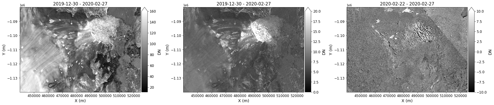
In this example, the anomaly can be useful for identifying area where the short-scale surface features are changing, which is important for analysis of ICESat data.
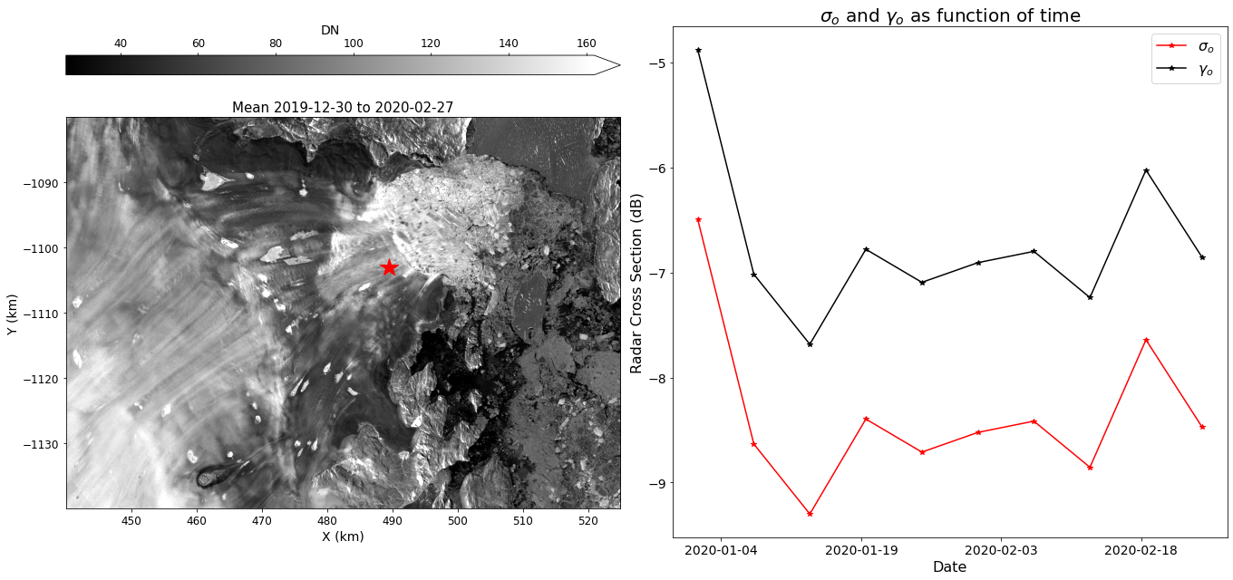
Interpolation
Values are easily interpolated from the image stack. For example, to plot \(\sigma_o\) and \(\gamma_o\) for the center of the image:
fig, axes = plt.subplots(1, 2, figsize=(19, 9))
#
# Display image mean
mean.displayImageForDate(date='2020-02-28', ax=axes[0], percentile=99, colorBarPosition='top',
title=f'Mean {mean.time1.strftime("%Y-%m-%d")} to {mean.time2.strftime("%Y-%m-%d")}',
units='km', colorBarPad=.65)
axes[0].plot(xc, yc, 'r*', markersize=20)
#
# Interpolate time series at point xc, yc
sigma0Center = mySigma0Series.interp(xc, yc, units='km') # Return result as np array (default)
gamma0Center = np.squeeze(myGamma0Series.interp(xc, yc, units='km', returnXR=True)) # Return results a Xarray
#
# Plot point results
axes[1].plot(mySigma0Series.time, sigma0Center, 'r*-', label='$\sigma_o$')
axes[1].plot(gamma0Center.time, gamma0Center, 'k*-', label='$\gamma_o$')
#
# Pretty up plot
axes[1].legend(fontsize=16)
axes[1].set_title('$\sigma_o$ and $\gamma_o$ as function of time', fontsize=20)
axes[1].xaxis.set_major_locator(plt.MaxNLocator(4)) # Reduce tick density
axes[1].set_xlabel('Date', fontsize=16)
axes[1].set_ylabel('Radar Cross Section (dB)', fontsize=16);
axes[1].tick_params(axis='both', labelsize=14)
fig.tight_layout()
Terminus Positions
Annual Terminus positions (with some gaps) for most of Greenlands glaciers are available at NSIDC in shape files.
myTerminusUrls = grimp.cmrUrls(mode='terminus') # mode image restricts search to the image products
myTerminusUrls.initialSearch()
myTerminusUrls.getURLS()
['https://n5eil01u.ecs.nsidc.org/DP4/MEASURES/NSIDC-0642.002/2000.09.30/termini_2000_2001_v02.0.shp',
'https://n5eil01u.ecs.nsidc.org/DP4/MEASURES/NSIDC-0642.002/2005.12.24/termini_2005_2006_v02.0.shp',
'https://n5eil01u.ecs.nsidc.org/DP4/MEASURES/NSIDC-0642.002/2007.01.06/termini_2006_2007_v02.0.shp',
'https://n5eil01u.ecs.nsidc.org/DP4/MEASURES/NSIDC-0642.002/2007.11.22/termini_2007_2008_v02.0.shp',
'https://n5eil01u.ecs.nsidc.org/DP4/MEASURES/NSIDC-0642.002/2009.01.04/termini_2008_2009_v02.0.shp',
'https://n5eil01u.ecs.nsidc.org/DP4/MEASURES/NSIDC-0642.002/2013.01.15/termini_2012_2013_v02.0.shp',
'https://n5eil01u.ecs.nsidc.org/DP4/MEASURES/NSIDC-0642.002/2015.02.07/termini_2014_2015_v02.0.shp',
'https://n5eil01u.ecs.nsidc.org/DP4/MEASURES/NSIDC-0642.002/2016.02.02/termini_2015_2016_v02.0.shp',
'https://n5eil01u.ecs.nsidc.org/DP4/MEASURES/NSIDC-0642.002/2017.02.01/termini_2016_2017_v02.0.shp',
'https://n5eil01u.ecs.nsidc.org/DP4/MEASURES/NSIDC-0642.002/2018.02.02/termini_2017_2018_v02.0.shp',
'https://n5eil01u.ecs.nsidc.org/DP4/MEASURES/NSIDC-0642.002/2019.02.03/termini_2018_2019_v02.0.shp',
'https://n5eil01u.ecs.nsidc.org/DP4/MEASURES/NSIDC-0642.002/2020.02.04/termini_2019_2020_v02.0.shp',
'https://n5eil01u.ecs.nsidc.org/DP4/MEASURES/NSIDC-0642.002/2021.02.04/termini_2020_2021_v02.0.shp']
These data can be read directly from NSIDC using GDAL’s Virtual File System (vsicurl) as though they existed locally on disk. To this, we need to:
append the prefix,
/vsicurl/&url=, to the url, andGDAL_HTTP_COOKIEFILEandGDAL_HTTP_COOKIEJARenvironment variables are set as shown above, andMake sure a
.netrcwith username and password exist (this file will be created as part of the login process above).
With the amended link, each shape file can be read as geopandas data frame:
myShapes = {}
#
# Look over list of urls
for url in myTerminusUrls.getURLS():
print('.', end='')
year = os.path.basename(url).split('_')[1] # Extract year from name
myShapes[year] = gpd.read_file(f'/vsicurl/&url={url}') # Add terminus to data frame
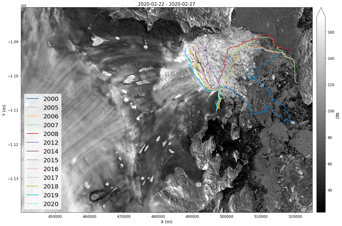
We can now plot the terminus locations for this glacier over the image.
fig, ax = plt.subplots(1, 1, figsize=(18, 14))
colors = plt.cm.tab20(np.linspace(0, 1, len(myShapes))).copy()
# Plot basemap
myImageSeries.displayImageForDate(date='2020-02-28', ax=ax, percentile=99, midDate=False, colorBarSize='3%', colorBarPad=.2) # Percentile clips range at 1-to-99%
box = shapely.geometry.Polygon([(x * 1000, y * 1000) for x, y in zip(xbox, ybox)])
# Plot each terminus
for key, color in zip(myShapes, colors):
# Find the terminus location that intersects the box
myShapes[key][myShapes[key]['geometry'].intersects(box)].plot(ax=ax, label=key, color=color, linewidth=2)
ax.legend(loc='lower left', fontsize=20);
GrIMP Summary
The examples above illustrate how image data for an area of interest can be extracted from the much larger remote NSIDC-0723 data set.
We used a relatively short time series, but the full data set for an area this size can be downloaded in a matter of several minutes.
More notebooks for working with GrIMP data are available here.
SlideRule
Introduction
SlideRule is an on-demand science data processing service that runs in on Amazon Web Services and responds to REST API calls to process and return science results. SlideRule was designed to enable researchers and other data systems to have low-latency access to custom-generated, high-level, analysis-ready data products using processing parameters supplied at the time of the request.
The SlideRule ICESat-2 plug-in is a cloud-optimized version of the ATL06 algorithm that can process the lower-level ATL03 geolocated photon height data products hosted on AWS by the NSIDC DAAC. This work supports science applications for the NASA Ice Cloud and land Elevation Satellite-2 (ICESat-2) mission.
Documentation for using SlideRule is available from the project website
Q: What does SlideRule ICESat-2 actually do?
SlideRule creates a simplified version of the ICESat-2 ATL06 land ice height product that can be adjusted to suit different needs. SlideRule let’s you create customized ICESat-2 segment heights directly from the photon height data anywhere on the globe, on-demand and quickly.
Jupyter and SlideRule
Jupyter widgets are used to set parameters for the SlideRule API.
Regions of interest for submitting to SlideRule are drawn on a leaflet map. Multiple regions of interest can be submitted at a given time.
The results from SlideRule can be displayed on the interactive leaflet map along with additional contextual layers.
Initiate SlideRule API
Sets the URL for accessing the SlideRule service
Builds a table of servers available for processing data
# set the url for the sliderule service
# set the logging level
sliderule.icesat2.init("icesat2sliderule.org", loglevel=logging.WARNING)
Set options for making science data processing requests to SlideRule
SlideRule follows a streamlined version of the ATL06 land ice height algorithm.
SlideRule also can use different sources for photon classification before calculating the average segment height.
This is useful for cases where there may be a vegetated canopy affecting the spread of the photon returns.
ATL03 photon confidence values, based on algorithm-specific classification types for land, ocean, sea-ice, land-ice, or inland water
ATL08 Land and Vegetation Height product photon classification
Experimental YAPC (Yet Another Photon Classification) photon-density-based classification
# display widgets for setting SlideRule parameters
SRwidgets = sliderule.ipysliderule.widgets()
# show widgets
widgets.VBox([
SRwidgets.asset,
SRwidgets.release,
SRwidgets.surface_type,
SRwidgets.length,
SRwidgets.step,
SRwidgets.confidence,
SRwidgets.land_class,
SRwidgets.iteration,
SRwidgets.spread,
SRwidgets.count,
SRwidgets.window,
SRwidgets.sigma
])
Interactive Mapping with Leaflet
There are 3 projections available within SlideRule for mapping
The interactive maps within the SlideRule python API are build upon ipyleaflet, which are Jupyter and python bindings for the fantastic Leaflet javascript library.
Leaflet Basemaps and Layers
There are also contextual layers available for each projection.
Global (Web Mercator, EPSG:3857)
North (Alaska Polar Stereographic, EPSG:5936)
South (Antarctic Polar Stereographic, EPSG:3031)
In addition, most xyzservice providers can be added as contextual layers to the global Web Mercator maps
widgets.VBox([SRwidgets.projection, SRwidgets.layers])
Select regions of interest for submitting to SlideRule
Here, we create polygons or bounding boxes for our regions of interest. This map is also our viewer for inspecting our SlideRule ICESat-2 data returns.
# create ipyleaflet map in specified projection
m = sliderule.ipysliderule.leaflet(SRwidgets.projection.value)
m.add_layer(layers=SRwidgets.layers.value)
# Comment this section out if you want to draw your own polygon!
# ---
box = shapely.geometry.Polygon([(-108.3,38.9), (-108.0,38.9), (-108.0,39.1), (-108.3, 39.1)])
geobox = gpd.GeoDataFrame(geometry=[box], crs='EPSG:4326')
default_polygon = sliderule.io.from_geodataframe(geobox)
geodata = ipyleaflet.GeoData(geo_dataframe=geobox)
m.map.add_layer(geodata)
# ---
m.map
Build and transmit requests to SlideRule
SlideRule will query the NASA Common Metadata Repository (CMR) for ATL03 data within our region of interest
When using the
nsidc-s3asset, the ICESat-2 ATL03 data are then accessed from the NSIDC AWS s3 bucket inus-west-2The ATL03 granules is spatially subset within SlideRule to our exact region of interest
SlideRule then uses our specified parameters to calculate average height segments from the ATL03 data in parallel
The completed data is streamed concurrently back and combined into a geopandas GeoDataFrame within the Python client
%%time
# sliderule asset and data release
asset = SRwidgets.asset.value
release = SRwidgets.release.value
# build sliderule parameters using latest values from widget
params = {
# surface type: 0-land, 1-ocean, 2-sea ice, 3-land ice, 4-inland water
"srt": SRwidgets.surface_type.index,
# length of ATL06-SR segment in meters
"len": SRwidgets.length.value,
# step distance for successive ATL06-SR segments in meters
"res": SRwidgets.step.value,
# confidence level for PE selection
"cnf": SRwidgets.confidence.value,
# ATL08 land surface classifications
"atl08_class": list(SRwidgets.land_class.value),
# maximum iterations, not including initial least-squares-fit selection
"maxi": SRwidgets.iteration.value,
# minimum along track spread
"ats": SRwidgets.spread.value,
# minimum PE count
"cnt": SRwidgets.count.value,
# minimum height of PE window in meters
"H_min_win": SRwidgets.window.value,
# maximum robust dispersion in meters
"sigma_r_max": SRwidgets.sigma.value
}
# create an empty geodataframe
gdf = sliderule.icesat2.__emptyframe()
# for each region of interest
all_regions = m.regions + default_polygon
for poly in all_regions:
# add polygon from map to sliderule parameters
params["poly"] = poly
# make the request to the SlideRule (ATL06-SR) endpoint
# and pass it the request parameters to request ATL06 Data
gdf = gdf.append(sliderule.icesat2.atl06p(params, asset, version=release))
CPU times: user 2.03 s, sys: 122 ms, total: 2.16 s
Wall time: 8.67 s
Review GeoDataFrame output
Can inspect the columns, number of returns and returns at the top of the GeoDataFrame.
See the ICESat-2 documentation for descriptions of each column
print(f'Returned {gdf.shape[0]} records')
gdf.head()
Returned 52631 records
| geometry | n_fit_photons | segment_id | h_sigma | pflags | rms_misfit | gt | delta_time | dh_fit_dy | cycle | h_mean | w_surface_window_final | spot | rgt | dh_fit_dx | distance | |
|---|---|---|---|---|---|---|---|---|---|---|---|---|---|---|---|---|
| 2018-10-17 22:31:18.138126884 | POINT (-108.29591 38.96142) | 15.0 | 216145.0 | 0.032286 | 0.0 | 0.080394 | 50.0 | 2.505068e+07 | 0.0 | 1.0 | 1744.120421 | 3.0 | 6.0 | 295.0 | 0.010093 | 4.334658e+06 |
| 2018-10-17 22:31:18.140942400 | POINT (-108.29593 38.96160) | 29.0 | 216146.0 | 0.016800 | 0.0 | 0.090111 | 50.0 | 2.505068e+07 | 0.0 | 1.0 | 1744.304732 | 3.0 | 6.0 | 295.0 | 0.005912 | 4.334678e+06 |
| 2018-10-17 22:31:18.143757660 | POINT (-108.29596 38.96178) | 39.0 | 216147.0 | 0.016053 | 0.0 | 0.099148 | 50.0 | 2.505068e+07 | 0.0 | 1.0 | 1744.457181 | 3.0 | 6.0 | 295.0 | 0.006901 | 4.334698e+06 |
| 2018-10-17 22:31:18.146572856 | POINT (-108.29598 38.96196) | 31.0 | 216148.0 | 0.019942 | 0.0 | 0.102734 | 50.0 | 2.505068e+07 | 0.0 | 1.0 | 1744.538714 | 3.0 | 6.0 | 295.0 | 0.000049 | 4.334718e+06 |
| 2018-10-17 22:31:18.149388076 | POINT (-108.29600 38.96214) | 21.0 | 216149.0 | 0.030903 | 0.0 | 0.135803 | 50.0 | 2.505068e+07 | 0.0 | 1.0 | 1744.464954 | 3.0 | 6.0 | 295.0 | -0.005180 | 4.334738e+06 |
Add GeoDataFrame to map
For stability of the leaflet map, SlideRule will as a default limit the plot to have up to 10000 points from the GeoDataFrame
GeoDataFrames can be plotted in any available matplotlib colormap
widgets.VBox([
SRwidgets.variable,
SRwidgets.cmap,
SRwidgets.reverse,
])
#%matplotlib inline
m.GeoData(gdf, column_name=SRwidgets.variable.value, cmap=SRwidgets.colormap,
max_plot_points=10000, tooltip=True, colorbar=True)
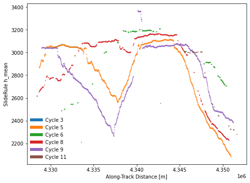
Create plots for a single track
# selection for reference ground track
RGTs = [str(int(x)) for x in gdf.rgt.unique()]
SRwidgets.rgt = widgets.Dropdown(
options=RGTs,
value=RGTs[1], # You can change this with the pull-down widget below!
description="RGT:",
description_tooltip="RGT: Reference Ground Track to plot",
disabled=False
)
# selection for ground track
ground_track_options = ["gt1l","gt1r","gt2l","gt2r","gt3l","gt3r"]
SRwidgets.ground_track = widgets.Dropdown(
options=ground_track_options,
value='gt1l',
description="Track:",
description_tooltip="Track: Ground Track to plot",
disabled=False
)
widgets.VBox([
SRwidgets.rgt,
SRwidgets.ground_track,
])
def cycles_plot(gdf, **kwargs):
"""Creates plots of SlideRule outputs
"""
# default keyword arguments
kwargs.setdefault('ax', None)
kwargs.setdefault('legend', False)
kwargs.setdefault('column_name', 'h_mean')
kwargs.setdefault('cycle_start', 3)
# variable to plot
column = kwargs['column_name']
# reference ground track and ground track
ground_track_dict = dict(gt1l=10,gt1r=20,gt2l=30,gt2r=40,gt3l=50,gt3r=60)
RGT = int(SRwidgets.rgt.value)
GT = int(ground_track_dict[SRwidgets.ground_track.value])
# skip plot creation if no values are entered
if (RGT == 0) or (GT == 0):
return
# create figure axis
if kwargs['ax'] is None:
fig,ax = plt.subplots(num=1, figsize=(8,6))
else:
ax = kwargs['ax']
# list of legend elements
legend_elements = []
# cycles: along-track plot showing all available cycles
# for each unique cycles
for cycle in gdf['cycle'].unique():
# skip cycles with significant off pointing
if (cycle < kwargs['cycle_start']):
continue
# reduce data frame to RGT, ground track and cycle
df = gdf[(gdf['rgt'] == RGT) & (gdf['gt'] == GT) &
(gdf['cycle'] == cycle)]
if not any(df[column].values):
continue
# plot reduced data frame
l, = ax.plot(df['distance'].values,
df[column].values, marker='.', lw=0, ms=1.5)
legend_elements.append(matplotlib.lines.Line2D([0], [0],
color=l.get_color(), lw=6,
label='Cycle {0:0.0f}'.format(cycle)))
# add axes labels
ax.set_xlabel('Along-Track Distance [m]')
ax.set_ylabel(f'SlideRule {column}')
# create legend
if kwargs['legend']:
lgd = ax.legend(handles=legend_elements, loc=3, frameon=True)
lgd.get_frame().set_alpha(1.0)
lgd.get_frame().set_edgecolor('white')
if kwargs['ax'] is None:
# show the figure
plt.tight_layout()
#%matplotlib widget
# create figure axis
fig,ax2 = plt.subplots(num=2, figsize=(8,6))
# default is to skip cycles with significant off-pointing
cycles_plot(gdf, ax=ax2, kind='cycles', cycle_start=3, legend=True)
Save GeoDataFrame to output file
pytables HDF5: easily read back as a Geopandas GeoDataFrame
netCDF: interoperable with other programs
display(SRwidgets.filesaver)
# append sliderule api version to attributes
version = sliderule.icesat2.get_version()
params['version'] = version['icesat2']['version']
params['commit'] = version['icesat2']['commit']
# save to file in format (HDF5 or netCDF)
sliderule.io.to_file(gdf, SRwidgets.file,
format=SRwidgets.format,
driver='pytables',
parameters=params,
regions=m.regions,
verbose=True)
ATL06-SR_20220414234910_004.h5
['n_fit_photons', 'segment_id', 'h_sigma', 'pflags', 'rms_misfit', 'gt', 'delta_time', 'dh_fit_dy', 'cycle', 'h_mean', 'w_surface_window_final', 'spot', 'rgt', 'dh_fit_dx', 'distance', 'latitude', 'longitude']
Read GeoDataFrame from input file
display(SRwidgets.fileloader)
print(SRwidgets.file)
# read from file in format (HDF5 or netCDF)
gdf = sliderule.io.from_file(SRwidgets.file,
format=SRwidgets.format,
driver='pytables')
ATL06-SR_20220414234910_004.h5
Review GeoDataFrame input from file
gdf.head()
| n_fit_photons | segment_id | h_sigma | pflags | rms_misfit | gt | delta_time | dh_fit_dy | cycle | h_mean | w_surface_window_final | spot | rgt | dh_fit_dx | distance | geometry | |
|---|---|---|---|---|---|---|---|---|---|---|---|---|---|---|---|---|
| 2018-10-17 22:31:18.138126884 | 15.0 | 216145.0 | 0.032286 | 0.0 | 0.080394 | 50.0 | 2.505068e+07 | 0.0 | 1.0 | 1744.120421 | 3.0 | 6.0 | 295.0 | 0.010093 | 4.334658e+06 | POINT (-108.29591 38.96142) |
| 2018-10-17 22:31:18.140942400 | 29.0 | 216146.0 | 0.016800 | 0.0 | 0.090111 | 50.0 | 2.505068e+07 | 0.0 | 1.0 | 1744.304732 | 3.0 | 6.0 | 295.0 | 0.005912 | 4.334678e+06 | POINT (-108.29593 38.96160) |
| 2018-10-17 22:31:18.143757660 | 39.0 | 216147.0 | 0.016053 | 0.0 | 0.099148 | 50.0 | 2.505068e+07 | 0.0 | 1.0 | 1744.457181 | 3.0 | 6.0 | 295.0 | 0.006901 | 4.334698e+06 | POINT (-108.29596 38.96178) |
| 2018-10-17 22:31:18.146572856 | 31.0 | 216148.0 | 0.019942 | 0.0 | 0.102734 | 50.0 | 2.505068e+07 | 0.0 | 1.0 | 1744.538714 | 3.0 | 6.0 | 295.0 | 0.000049 | 4.334718e+06 | POINT (-108.29598 38.96196) |
| 2018-10-17 22:31:18.149388076 | 21.0 | 216149.0 | 0.030903 | 0.0 | 0.135803 | 50.0 | 2.505068e+07 | 0.0 | 1.0 | 1744.464954 | 3.0 | 6.0 | 295.0 | -0.005180 | 4.334738e+06 | POINT (-108.29600 38.96214) |
Region of Interest from SAR imagery
# bounding box for SAR images
bbox = {'minx': 440000, 'miny': -1140000, 'maxx': 525000, 'maxy': -1080000}
xbox = np.array([bbox[x] for x in ['minx', 'maxx', 'maxx', 'minx']])
ybox = np.array([bbox[y] for y in ['miny', 'miny', 'maxy', 'maxy']])
# create shapely polygon of bounding box and convert to geodataframe
box = shapely.geometry.Polygon([(x, y) for x, y in zip(xbox, ybox)])
geobox = gpd.GeoDataFrame(geometry=[box], crs='EPSG:3413')
# convert to sliderule request polygons
polygons = sliderule.io.from_geodataframe(geobox)
Build and transmit request to SlideRule for SAR bounding box
%%time
# sliderule asset and data release
asset = SRwidgets.asset.value
release = SRwidgets.release.value
# build sliderule parameters
params = {
"srt": 3,
"len": 20,
"res": 10,
"cnf": 1,
"maxi": 6,
"ats": 10,
"cnt": 10,
"H_min_win": 3,
"sigma_r_max": 5,
# add start and end time based on SAR range
't0': '2020-01-01T00:00:00Z',
't1': '2020-02-24T23:59:59Z'
}
# create an empty geodataframe
gdf = sliderule.icesat2.__emptyframe()
# for each region of interest
for poly in polygons:
# add polygon from geodataframe
params["poly"] = poly
# make the request to the SlideRule (ATL06-SR) endpoint
# and pass it the request parameters to request ATL06 Data
gdf = gdf.append(sliderule.icesat2.atl06p(params, asset, version=release))
CPU times: user 14 s, sys: 690 ms, total: 14.7 s
Wall time: 16.1 s
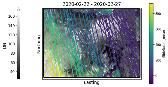
Create a static map with SlideRule returns
geopandas GeoDataFrames can be transformed to different Coordinate Reference Systems (CRS) using the to_crs() function.
Here, we’ll make a static map of Greenland containing our SlideRule returns and use our SAR imagery as a basemap.
fig,ax1 = plt.subplots(num=1, figsize=(9,5))
# plot SAR image as basemap
# Percentile clips range at 1-to-99%
myImageSeries.displayImageForDate(date='2020-02-28', ax=ax1, percentile=99,
midDate=False, colorBarSize='3%', colorBarPosition='left', colorBarPad=1.0)
# add sliderule returns
gdf3413 = gdf.to_crs('EPSG:3413')
column = 'h_mean'
label = f'SlideRule {column}'
sc = gdf3413.plot(ax=ax1, markersize=0.5,
column=column, cmap=SRwidgets.colormap, legend=True,
legend_kwds=dict(label=label, shrink=0.95))
xmin,ymin,xmax,ymax = gdf3413.total_bounds
# plot each region of interest
regions = []
for poly in polygons:
lon,lat = sliderule.io.from_region(poly)
regions.append(shapely.geometry.Polygon(zip(lon,lat)))
gs = gpd.GeoSeries(regions,crs='EPSG:4326').to_crs('EPSG:3413')
gs.plot(ax=ax1,facecolor='none',edgecolor='black',lw=3)
# set x and y limits
ax1.set_xlim(xmin-1e3,xmax+1e3)
ax1.set_ylim(ymin-1e3,ymax+1e3)
ax1.set_aspect('equal', adjustable='box')
# remove x and y ticks
ax1.set_xticks([])
ax1.set_yticks([])
# add x and y labels
ax1.set_xlabel('Easting')
ax1.set_ylabel('Northing')
Text(114.97966019417476, 0.5, 'Northing')
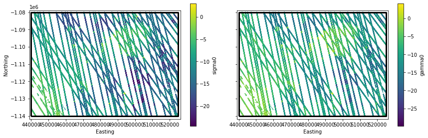
Applying Concepts: Interpolation to SlideRule Returns
We’ll plot \(\sigma_o\) and \(\gamma_o\) interpolated to the locations of the SlideRule returns
These routines could also be applied to interpolate velocities (stay tuned to the next Data Integration Tutorial).
# extract sliderule points
SRx = gdf3413.geometry.x.values
SRy = gdf3413.geometry.y.values
# Interpolate SAR time series for sliderule points
SRsigma0 = mySigma0Series.interp(SRx, SRy, units='m')
SRgamma0 = myGamma0Series.interp(SRx, SRy, units='m')
%%time
# NOTE: generating this plot takes a while!
fig,ax3 = plt.subplots(num=3, ncols=2, sharex=True, sharey=True, figsize=(12,4))
# add sigma0 and gamma0 interpolated to sliderule returns
gdf3413 = gdf.to_crs('EPSG:3413')
gdf3413['sigma0'] = SRsigma0[0,:]
gdf3413['gamma0'] = SRgamma0[0,:]
label = f'SlideRule {SRwidgets.variable.value}'
gdf3413.plot(ax=ax3[0], markersize=0.5,
column='sigma0', cmap=SRwidgets.colormap, legend=True,
legend_kwds=dict(label='sigma0', shrink=0.95))
gdf3413.plot(ax=ax3[1], markersize=0.5,
column='gamma0', cmap=SRwidgets.colormap, legend=True,
legend_kwds=dict(label='gamma0', shrink=0.95))
xmin,ymin,xmax,ymax = gdf3413.total_bounds
# plot each region of interest
regions = []
for poly in polygons:
lon,lat = sliderule.io.from_region(poly)
regions.append(shapely.geometry.Polygon(zip(lon,lat)))
gs = gpd.GeoSeries(regions,crs='EPSG:4326').to_crs('EPSG:3413')
gs.plot(ax=ax3[0],facecolor='none',edgecolor='black',lw=3)
gs.plot(ax=ax3[1],facecolor='none',edgecolor='black',lw=3)
# set x and y limits
ax3[0].set_xlim(xmin-1e3,xmax+1e3)
ax3[0].set_ylim(ymin-1e3,ymax+1e3)
ax3[0].set_aspect('equal', adjustable='box')
# add x and y labels
ax3[0].set_xlabel('Easting')
ax3[1].set_xlabel('Easting')
ax3[0].set_ylabel('Northing')
# adjust subplot and show
fig.subplots_adjust(left=0.06,right=0.98,bottom=0.08,top=0.98,wspace=0.1)
CPU times: user 1min 35s, sys: 579 ms, total: 1min 35s
Wall time: 1min 35s
Summary
You have seen how we can search for GrIMP datasets, open them into xarray datasets, and explore the datasets. You’ve also seen how to make requests to SlideRule for elevation data from ICESat-2, and exploring the data interactively.