This tutorial is meant to show some examples of the standard land-ice data products put out by the ICESat-2 project. It is not a comprehensive look at all the products, nor does it document all the features available in the product is shows. Rather, it presents some tools for looking at the data, and shows how the information flows between land-ice products.
Demonstrate basic HDF-5 product structures of ICESat-2 standard data products
Demonstrate the flow of information from the lowest-level products to the highest-level products (or vice versa)
Data search using geographic regions and file names using icePyx
File-level data access from NSIDC
Photon data access using SlideRule
# import packages:importnumpyasnp# Numeric Pythonimportmatplotlib.pyplotasplt# Plotting routinesimporth5py# general HDF5 reading/writing libraryimportrioxarrayasrx# Package to read raster data from hdf5 filesfrompyprojimportTransformer,CRS# libraries to allow coordinate transformsimportglob# Package to locate files on diskimportos# File-level utilitiesimportre# regular expressions for string interpretationimporticepyxasipx# Package to interact with ICESat-2 online resourcesfromslideruleimporticesat2# Package for online ICESat-2 processing
#Please note: This tutorial is best run in interactive mode,# but is archived with the interactive section disabled.# To enable interactive mode, comment the next line, and uncomment the second line:%matplotlib inline
#%matplotlib widget %config InlineBackend.figure_format = 'retina'
0. Get access to earthdata using a .netrc file. You’ll need to do this to run the notebook!
We will need to generate a (hidden) .netrc file in our local directory. The NASA Openscapes 2021 Cloud Hackathon came up with a function that does this painlessly. You’ll only have to run this once on each computer you use for this tutorial. If you’re running interactively, you’ll have to uncomment two lines in the next cell and run that cell.
#DEFAULT: to generate the rendered tutorial for the book. Comment these two lines if you are running interactivelyHOST='https://urs.earthdata.nasa.gov'ipx.core.Earthdata.Earthdata('uwhackweek','hackweekadmin@gmail.com',HOST).login()# If you are running interactively, uncomment these two lines, and run this cell!#from setup_earthdata_netrc import setup_earthdata_netrc#setup_earthdata_netrc()
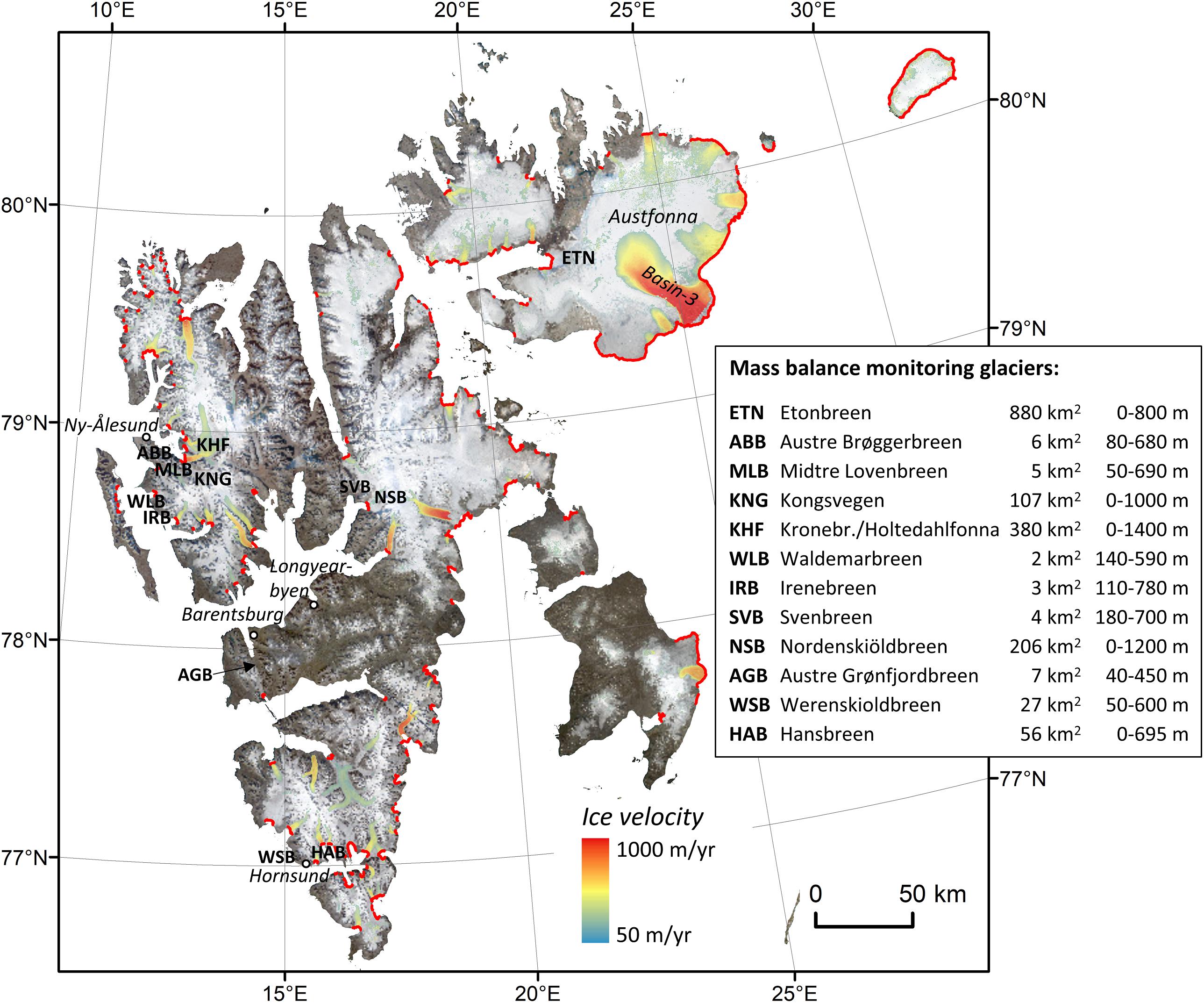
We will be looking at Svalbard in the Norwegian Arctic, focusing on the massive surge from the Austfonna ice cap. This started in 2010, and the ice cap is still adjusting to the rapid loss of ice, so we expect to see large thinning rates in the area affected by the surge. We will use the ICESat-2 ATL15 product for a look at the mass-loss pattern over the last three years.
ATL15 provides a high-level map of how ice-surface heights have changed. It supplies grids of surface-height differences relative to a January-2020 reference surface, at quarter-year, 1-km resolution. It comes in subsets for different polar glaciated regions:
The Antarctic and Greenland full-resolution granules are large, but the smaller regions () are compact files that are quick to download.
We’ll download these files directly from NSIDC using the unix ‘wget’ command. You’ll need to have your login credentials set up for this to work. Please check near the top of this tutorial (section zero) for help with this.
Once our credentials are set up, we can use wget to download the ATL15 Svalbard granule:
# Download (-nc = "no clobber" if it already existsds_url='https://n5eil01u.ecs.nsidc.org/ATLAS/ATL15.001/2019.03.29/ATL15_SV_0311_01km_001_01.nc'! wget -nc {ds_url} -O /tmp/ATL15_SV_0311_01km_001_01.nc
302 Found
Location: https://urs.earthdata.nasa.gov/oauth/authorize?app_type=401&client_id=_JLuwMHxb2xX6NwYTb4dRA&response_type=code&redirect_uri=https%3A%2F%2Fn5eil01u.ecs.nsidc.org%2FOPS%2Fredirect&state=aHR0cDovL241ZWlsMDF1LmVjcy5uc2lkYy5vcmcvQVRMQVMvQVRMMTUuMDAxLzIwMTkuMDMuMjkvQVRMMTVfU1ZfMDMxMV8wMWttXzAwMV8wMS5uYw [following]
--2022-04-14 23:40:37--  https://urs.earthdata.nasa.gov/oauth/authorize?app_type=401&client_id=_JLuwMHxb2xX6NwYTb4dRA&response_type=code&redirect_uri=https%3A%2F%2Fn5eil01u.ecs.nsidc.org%2FOPS%2Fredirect&state=aHR0cDovL241ZWlsMDF1LmVjcy5uc2lkYy5vcmcvQVRMQVMvQVRMMTUuMDAxLzIwMTkuMDMuMjkvQVRMMTVfU1ZfMDMxMV8wMWttXzAwMV8wMS5uYw
Resolving urs.earthdata.nasa.gov (urs.earthdata.nasa.gov)... 198.118.243.33, 2001:4d0:241a:4081::89
Connecting to urs.earthdata.nasa.gov (urs.earthdata.nasa.gov)|198.118.243.33|:443... connected.
HTTP request sent, awaiting response... 401 Unauthorized
Authentication selected: Basic realm="Please enter your Earthdata Login credentials. If you do not have a Earthdata Login, create one at https://urs.earthdata.nasa.gov//users/new"
Reusing existing connection to urs.earthdata.nasa.gov:443.
HTTP request sent, awaiting response...
302 Found
Location: https://n5eil01u.ecs.nsidc.org/OPS/redirect?code=8757088a878353ef27c5ac728d629a10cf16e1438f4bee19fa741d0c89ab893e&state=aHR0cDovL241ZWlsMDF1LmVjcy5uc2lkYy5vcmcvQVRMQVMvQVRMMTUuMDAxLzIwMTkuMDMuMjkvQVRMMTVfU1ZfMDMxMV8wMWttXzAwMV8wMS5uYw [following]
--2022-04-14 23:40:37--  https://n5eil01u.ecs.nsidc.org/OPS/redirect?code=8757088a878353ef27c5ac728d629a10cf16e1438f4bee19fa741d0c89ab893e&state=aHR0cDovL241ZWlsMDF1LmVjcy5uc2lkYy5vcmcvQVRMQVMvQVRMMTUuMDAxLzIwMTkuMDMuMjkvQVRMMTVfU1ZfMDMxMV8wMWttXzAwMV8wMS5uYw
Connecting to n5eil01u.ecs.nsidc.org (n5eil01u.ecs.nsidc.org)|128.138.97.102|:443...
connected.
HTTP request sent, awaiting response...
302 Found
Location: https://n5eil01u.ecs.nsidc.org/ATLAS/ATL15.001/2019.03.29/ATL15_SV_0311_01km_001_01.nc [following]
--2022-04-14 23:40:38--  https://n5eil01u.ecs.nsidc.org/ATLAS/ATL15.001/2019.03.29/ATL15_SV_0311_01km_001_01.nc
Connecting to n5eil01u.ecs.nsidc.org (n5eil01u.ecs.nsidc.org)|128.138.97.102|:443...
connected.
HTTP request sent, awaiting response...
200 OK
Length: 11413193 (11M) [application/x-netcdf]
Saving to: ‘/tmp/ATL15_SV_0311_01km_001_01.nc’


          /tmp/ATL1   0%[                    ]       0  --.-KB/s
If the previous slide did not download data, you may need to revisit the commented cell just after section zero (0. Get access to earthdata using a .netrc file.) You’ll need to do this to run the notebook!
The data we want to look at are in the delta_h group, and we can see the structure of the product by opening it with rioxarray:
This data set (ATL15) contains seasonal, annual, and biennial gridded land ice elevation change.
identifier :
atl15_qa_util
pulse_rate :
10000 pps
type :
Spacecraft
wavelength :
532 nm
Description :
Describe the group
edition :
v1.0
publicationDate :
Feb 2020
title :
SET_BY_META
evaluationMethodType :
directInternal
measureDescription :
TBD
nameOfMeasure :
TBD
unitofMeasure :
TBD
value :
NOT_SET
scope :
NOT_SET
abstract :
The ICESat-2 ATL15 standard data product reports a land ice elevation change as comapred to an ice sheet digital elevation model (DEM).
characterSet :
utf8
creationDate :
2021-12-03T00:16:38.000000Z
credit :
The software that generates the ATL15 product was designed and implemented within the ICESat-2 Science Investigator-led Processing System at the NASA Goddard Space Flight Center in Greenbelt, Maryland.
fileName :
ATL15_SV_0311_01km_001_01.nc
language :
eng
originatorOrganizationName :
GSFC I-SIPS > ICESat-2 Science Investigator-led Processing System
purpose :
The purpose of ATL15 is to provide an IceSat-2 gridded satellite summary of height changes of land-based ice.
<?xml version="1.0" encoding="UTF-8"?>
<gmd:DS_Series
xmlns:eos="http://earthdata.nasa.gov/schema/eos"
xmlns:gco="http://www.isotc211.org/2005/gco"
xmlns:gmd="http://www.isotc211.org/2005/gmd"
xmlns:gmi="http://www.isotc211.org/2005/gmi"
xmlns:gml="http://www.opengis.net/gml/3.2"
xmlns:gmx="http://www.isotc211.org/2005/gmx"
xmlns:gsr="http://www.isotc211.org/2005/gsr"
xmlns:gss="http://www.isotc211.org/2005/gss"
xmlns:gts="http://www.isotc211.org/2005/gts"
xmlns:srv="http://www.isotc211.org/2005/srv"
xmlns:xlink="http://www.w3.org/1999/xlink"
xmlns:xs="http://www.w3.org/2001/XMLSchema"
xmlns:xsi="http://www.w3.org/2001/XMLSchema-instance"
xsi:schemaLocation="http://www.isotc211.org/2005/gmi http://cdn.earthdata.nasa.gov/iso/schema/1.0/ISO19115-2_EOS.xsd">
<gmd:composedOf gco:nilReason="inapplicable"/>
<gmd:seriesMetadata>
<gmi:MI_Metadata>
<gmd:fileIdentifier>
<gco:CharacterString>ATL15.001</gco:CharacterString>
</gmd:fileIdentifier>
<gmd:language>
<gco:CharacterString>eng</gco:CharacterString>
</gmd:language>
<gmd:characterSet>
<gmd:MD_CharacterSetCode codeList="http://cdn.earthdata.nasa.gov/iso/resources/Codelist/gmxCodelists.xml#MD_CharacterSetCode" codeListValue="utf8">utf8</gmd:MD_CharacterSetCode>
</gmd:characterSet>
<gmd:hierarchyLevel>
<gmd:MD_ScopeCode codeList="http://cdn.earthdata.nasa.gov/iso/resources/Codelist/gmxCodelists.xml#MD_ScopeCode" codeListValue="series">series</gmd:MD_ScopeCode>
</gmd:hierarchyLevel>
<gmd:contact>
<gmd:CI_ResponsibleParty>
<gmd:organisationName>
<gco:CharacterString>NSIDC DAAC > NASA National Snow and Ice Data Center Distributed Active Archive Center</gco:CharacterString>
</gmd:organisationName>
<gmd:contactInfo>
<gmd:CI_Contact id="NSIDC_DAAC_CONTACT_ID">
<gmd:phone>
<gmd:CI_Telephone>
<gmd:voice>
<gco:CharacterString>303-492-6199</gco:CharacterString>
</gmd:voice>
<gmd:facsimile>
<gco:CharacterString>303-492-2468</gco:CharacterString>
</gmd:facsimile>
</gmd:CI_Telephone>
</gmd:phone>
<gmd:address>
<gmd:CI_Address>
<gmd:deliveryPoint>
<gco:CharacterString>1540 30th St Campus Box 449</gco:CharacterString>
</gmd:deliveryPoint>
<gmd:city>
<gco:CharacterString>Boulder</gco:CharacterString>
</gmd:city>
<gmd:administrativeArea>
<gco:CharacterString>Colorado</gco:CharacterString>
</gmd:administrativeArea>
<gmd:postalCode>
<gco:CharacterString>80309-0449</gco:CharacterString>
</gmd:postalCode>
<gmd:country>
<gco:CharacterString>USA</gco:CharacterString>
</gmd:country>
<gmd:electronicMailAddress>
<gco:CharacterString>nsidc@nsidc.org</gco:CharacterString>
</gmd:electronicMailAddress>
</gmd:CI_Address>
</gmd:address>
<gmd:onlineResource>
<gmd:CI_OnlineResource>
<gmd:linkage>
<gmd:URL>http://nsidc.org/daac/</gmd:URL>
</gmd:linkage>
</gmd:CI_OnlineResource>
</gmd:onlineResource>
<gmd:hoursOfService>
<gco:CharacterString>9:00 A.M. to 5:00 P.M., U.S. Mountain Time, Monday through Friday, excluding U.S. holidays.</gco:CharacterString>
</gmd:hoursOfService>
<gmd:contactInstructions>
<gco:CharacterString>Contact by e-mail first</gco:CharacterString>
</gmd:contactInstructions>
</gmd:CI_Contact>
</gmd:contactInfo>
<gmd:role>
<gmd:CI_RoleCode codeList="http://cdn.earthdata.nasa.gov/iso/resources/Codelist/gmxCodelists.xml#CI_RoleCode" codeListValue="pointOfContact">pointOfContact</gmd:CI_RoleCode>
</gmd:role>
</gmd:CI_ResponsibleParty>
</gmd:contact>
<gmd:dateStamp>
<gco:Date>2015-10-15</gco:Date>
</gmd:dateStamp>
<gmd:metadataStandardName>
<gco:CharacterString>ISO 19115-2 Geographic information - Metadata - Part 2: Extensions for imagery and gridded data</gco:CharacterString>
</gmd:metadataStandardName>
<gmd:metadataStandardVersion>
<gco:CharacterString>ISO 19115-2:2009(E)</gco:CharacterString>
</gmd:metadataStandardVersion>
<gmd:identificationInfo>
<gmd:MD_DataIdentification>
<gmd:citation>
<gmd:CI_Citation>
<!-- ECS extracts the LongName from here -->
<!-- UMM-C expects the ShortName to precede the LongName separated by a > here -->
<gmd:title>
<gco:CharacterString>ATLAS/ICESat-2 L3B Seasonal, Annual, and Biennial Land Ice Height Change</gco:CharacterString>
</gmd:title>
<gmd:date>
<gmd:CI_Date>
<!-- ECS extracts the RevisionDate from here -->
<gmd:date>
<gco:Date>2021-06-07</gco:Date>
</gmd:date>
<gmd:dateType>
<gmd:CI_DateTypeCode codeList="http://cdn.earthdata.nasa.gov/iso/resources/Codelist/gmxCodelists.xml#CI_DateTypeCode" codeListValue="revision">revision</gmd:CI_DateTypeCode>
</gmd:dateType>
</gmd:CI_Date>
</gmd:date>
<!-- VersionID is expected to be here by the Base Reference Metadata Model document -->
<gmd:edition>
<gco:CharacterString>001</gco:CharacterString>
</gmd:edition>
<gmd:identifier>
<gmd:MD_Identifier>
<!-- ECS extracts the ShortName from here -->
<gmd:code>
<gco:CharacterString>ATL15</gco:CharacterString>
</gmd:code>
<gmd:description>
<gco:CharacterString>The ECS Short Name</gco:CharacterString>
</gmd:description>
</gmd:MD_Identifier>
</gmd:identifier>
<gmd:identifier>
<gmd:MD_Identifier>
<!-- ECS extracts the VersionID from here -->
<gmd:code>
<gco:CharacterString>001</gco:CharacterString>
</gmd:code>
<gmd:description>
<gco:CharacterString>The ECS Version ID</gco:CharacterString>
</gmd:description>
</gmd:MD_Identifier>
</gmd:identifier>
<gmd:identifier>
<gmd:MD_Identifier>
<!-- This field provides the Digital Object Identifier (DOI). -->
<gmd:code>
<gmx:Anchor xlink:actuate="onRequest" xlink:href="https://doi.org/10.5067/ATLAS/ATL15.001">doi:10.5067/ATLAS/ATL15.001</gmx:Anchor>
</gmd:code>
<gmd:codeSpace>
<gco:CharacterString>gov.nasa.esdis</gco:CharacterString>
</gmd:codeSpace>
<gmd:description>
<gco:CharacterString>A Digital Object Identifier (DOI)</gco:CharacterString>
</gmd:description>
</gmd:MD_Identifier>
</gmd:identifier>
<gmd:citedResponsibleParty>
<gmd:CI_ResponsibleParty>
<gmd:organisationName>
<gco:CharacterString>National Aeronautics and Space Administration (NASA)</gco:CharacterString>
</gmd:organisationName>
<gmd:role>
<gmd:CI_RoleCode codeList="http://www.isotc211.org/2005/resources/Codelist/gmxCodelists.xml#CI_RoleCode" codeListValue="resourceProvider">resourceProvider</gmd:CI_RoleCode>
</gmd:role>
</gmd:CI_ResponsibleParty>
</gmd:citedResponsibleParty>
<gmd:citedResponsibleParty>
<gmd:CI_ResponsibleParty>
<!-- ECS expects ProcessingCenter to be here -->
<gmd:organisationName>
<gco:CharacterString>GSFC I-SIPS > ICESat-2 Science Investigator-led Processing System</gco:CharacterString>
</gmd:organisationName>
<gmd:role>
<gmd:CI_RoleCode codeList="http://cdn.earthdata.nasa.gov/iso/resources/Codelist/gmxCodelists.xml#CI_RoleCode" codeListValue="originator">originator</gmd:CI_RoleCode>
</gmd:role>
</gmd:CI_ResponsibleParty>
</gmd:citedResponsibleParty>
<!-- ECS extracts the VersionDescription from here -->
<gmd:otherCitationDetails>
<gco:CharacterString>Initial version of the processing software</gco:CharacterString>
</gmd:otherCitationDetails>
</gmd:CI_Citation>
</gmd:citation>
<!-- ECS extracts the CollectionDescription from here -->
<gmd:abstract>
<gco:CharacterString>The ICESat-2 ATL15 standard data product reports a land ice elevation change as comapred to an ice sheet digital elevation model (DEM).</gco:CharacterString>
</gmd:abstract>
<gmd:purpose>
<gco:CharacterString>The purpose of ATL15 is to provide an IceSat-2 gridded satellite summary of height changes of land-based ice.</gco:CharacterString>
</gmd:purpose>
<gmd:credit>
<gco:CharacterString>The software that generates the ATL15 product was designed and implemented within the ICESat-2 Science Investigator-led Processing System at the NASA Goddard Space Flight Center in Greenbelt, Maryland.</gco:CharacterString>
</gmd:credit>
<gmd:status>
<gmd:MD_ProgressCode codeList="http://www.isotc211.org/2005/resources/Codelist/gmxCodelists.xml#MD_ProgressCode" codeListValue="onGoing">onGoing</gmd:MD_ProgressCode>
</gmd:status>
<gmd:pointOfContact>
<gmd:CI_ResponsibleParty>
<!-- ECS expects ArchiveCenter to be here -->
<gmd:organisationName>
<gco:CharacterString>NSIDC DAAC > NASA National Snow and Ice Data Center Distributed Active Archive Center</gco:CharacterString>
</gmd:organisationName>
<gmd:contactInfo xlink:href="#NSIDC_DAAC_CONTACT_ID"/>
<gmd:role>
<gmd:CI_RoleCode codeList="http://cdn.earthdata.nasa.gov/iso/resources/Codelist/gmxCodelists.xml#CI_RoleCode" codeListValue="distributor">distributor</gmd:CI_RoleCode>
</gmd:role>
</gmd:CI_ResponsibleParty>
</gmd:pointOfContact>
<gmd:resourceFormat>
<gmd:MD_Format>
<gmd:name>
<gco:CharacterString>HDF</gco:CharacterString>
</gmd:name>
<gmd:version>
<gco:CharacterString>5</gco:CharacterString>
</gmd:version>
</gmd:MD_Format>
</gmd:resourceFormat>
<gmd:descriptiveKeywords>
<gmd:MD_Keywords>
<gmd:keyword>
<gco:CharacterString>EARTH SCIENCE > CRYOSPHERE > GLACIERS/ICE SHEETS > GLACIER ELEVATION/ICE SHEET ELEVATION > NONE > NONE > NONE</gco:CharacterString>
</gmd:keyword>
<gmd:keyword>
<gco:CharacterString>EARTH SCIENCE > TERRESTRIAL HYDROSPHERE > GLACIERS/ICE SHEETS > GLACIER ELEVATION/ICE SHEET ELEVATION > NONE > NONE > NONE</gco:CharacterString>
</gmd:keyword>
<gmd:type>
<gmd:MD_KeywordTypeCode codeList="http://cdn.earthdata.nasa.gov/iso/resources/Codelist/gmxCodelists.xml#MD_KeywordTypeCode" codeListValue="theme">theme</gmd:MD_KeywordTypeCode>
</gmd:type>
<gmd:thesaurusName>
<gmd:CI_Citation>
<gmd:title>
<gco:CharacterString>NASA/GCMD Science Keywords</gco:CharacterString>
</gmd:title>
<gmd:date gco:nilReason="unknown"/>
<gmd:citedResponsibleParty>
<gmd:CI_ResponsibleParty id="GCMD_USO_ID">
<gmd:organisationName>
<gco:CharacterString>NASA Global Change Master Directory (GCMD) User Support Office</gco:CharacterString>
</gmd:organisationName>
<gmd:contactInfo>
<gmd:CI_Contact>
<gmd:phone gco:nilReason="missing"/>
<gmd:address>
<gmd:CI_Address>
<gmd:deliveryPoint>
<gco:CharacterString>NASA Global Change Master Directory, Goddard Space Flight Center</gco:CharacterString>
</gmd:deliveryPoint>
<gmd:city>
<gco:CharacterString>Greenbelt</gco:CharacterString>
</gmd:city>
<gmd:administrativeArea>
<gco:CharacterString>MD</gco:CharacterString>
</gmd:administrativeArea>
<gmd:postalCode>
<gco:CharacterString>20771</gco:CharacterString>
</gmd:postalCode>
<gmd:country>
<gco:CharacterString>USA</gco:CharacterString>
</gmd:country>
<gmd:electronicMailAddress>
<gco:CharacterString>gcmduso@gcmd.gsfc.nasa.gov</gco:CharacterString>
</gmd:electronicMailAddress>
</gmd:CI_Address>
</gmd:address>
<gmd:onlineResource>
<gmd:CI_OnlineResource>
<gmd:linkage>
<gmd:URL>http://gcmd.nasa.gov/</gmd:URL>
</gmd:linkage>
<gmd:protocol>
<gco:CharacterString>http</gco:CharacterString>
</gmd:protocol>
<gmd:applicationProfile>
<gco:CharacterString>web browser</gco:CharacterString>
</gmd:applicationProfile>
<gmd:name>
<gco:CharacterString>NASA Global Change Master Directory (GCMD)</gco:CharacterString>
</gmd:name>
<gmd:description>
<gco:CharacterString>Home Page</gco:CharacterString>
</gmd:description>
<gmd:function>
<gmd:CI_OnLineFunctionCode codeList="http://cdn.earthdata.nasa.gov/iso/resources/Codelist/gmxCodelists.xml#CI_OnLineFunctionCode" codeListValue="information">information</gmd:CI_OnLineFunctionCode>
</gmd:function>
</gmd:CI_OnlineResource>
</gmd:onlineResource>
<gmd:contactInstructions>
<gco:CharacterString>http://gcmd.nasa.gov/MailComments/MailComments.jsf?rcpt=gcmduso</gco:CharacterString>
</gmd:contactInstructions>
</gmd:CI_Contact>
</gmd:contactInfo>
<gmd:role>
<gmd:CI_RoleCode codeList="http://cdn.earthdata.nasa.gov/iso/resources/Codelist/gmxCodelists.xml#CI_RoleCode" codeListValue="custodian">custodian</gmd:CI_RoleCode>
</gmd:role>
</gmd:CI_ResponsibleParty>
</gmd:citedResponsibleParty>
<gmd:citedResponsibleParty>
<gmd:CI_ResponsibleParty id="GCMD_KEYWORDS_ID">
<gmd:organisationName>
<gco:CharacterString>Global Change Master Directory (GCMD)</gco:CharacterString>
</gmd:organisationName>
<gmd:contactInfo>
<gmd:CI_Contact>
<gmd:phone gco:nilReason="missing"/>
<gmd:address>
<gmd:CI_Address>
<gmd:deliveryPoint>
<gco:CharacterString>NASA Global Change Master Directory, Goddard Space Flight Center</gco:CharacterString>
</gmd:deliveryPoint>
<gmd:city>
<gco:CharacterString>Greenbelt</gco:CharacterString>
</gmd:city>
<gmd:administrativeArea>
<gco:CharacterString>MD</gco:CharacterString>
</gmd:administrativeArea>
<gmd:postalCode>
<gco:CharacterString>20771</gco:CharacterString>
</gmd:postalCode>
<gmd:country>
<gco:CharacterString>USA</gco:CharacterString>
</gmd:country>
<gmd:electronicMailAddress>
<gco:CharacterString>gcmduso@gcmd.gsfc.nasa.gov</gco:CharacterString>
</gmd:electronicMailAddress>
</gmd:CI_Address>
</gmd:address>
<gmd:onlineResource>
<gmd:CI_OnlineResource>
<gmd:linkage>
<gmd:URL>http://gcmd.nasa.gov/Resources/valids/</gmd:URL>
</gmd:linkage>
<gmd:protocol>
<gco:CharacterString>http</gco:CharacterString>
</gmd:protocol>
<gmd:applicationProfile>
<gco:CharacterString>web browser</gco:CharacterString>
</gmd:applicationProfile>
<gmd:name>
<gco:CharacterString>NASA Global Change Master Directory (GCMD) Keyword Page</gco:CharacterString>
</gmd:name>
<gmd:description>
<gco:CharacterString>This page describes the NASA GCMD Keywords, how to reference those keywords and provides download instructions.</gco:CharacterString>
</gmd:description>
<gmd:function>
<gmd:CI_OnLineFunctionCode codeList="http://cdn.earthdata.nasa.gov/iso/resources/Codelist/gmxCodelists.xml#CI_OnLineFunctionCode" codeListValue="download">download</gmd:CI_OnLineFunctionCode>
</gmd:function>
</gmd:CI_OnlineResource>
</gmd:onlineResource>
<gmd:contactInstructions>
<gco:CharacterString>http://gcmd.nasa.gov/MailComments/MailComments.jsf?rcpt=gcmduso</gco:CharacterString>
</gmd:contactInstructions>
</gmd:CI_Contact>
</gmd:contactInfo>
<gmd:role>
<gmd:CI_RoleCode codeList="http://cdn.earthdata.nasa.gov/iso/resources/Codelist/gmxCodelists.xml#CI_RoleCode" codeListValue="custodian">custodian</gmd:CI_RoleCode>
</gmd:role>
</gmd:CI_ResponsibleParty>
</gmd:citedResponsibleParty>
</gmd:CI_Citation>
</gmd:thesaurusName>
</gmd:MD_Keywords>
</gmd:descriptiveKeywords>
<gmd:descriptiveKeywords>
<gmd:MD_Keywords>
<gmd:keyword>
<gco:CharacterString>GEOGRAPHIC REGION > GLOBAL</gco:CharacterString>
</gmd:keyword>
<gmd:type>
<gmd:MD_KeywordTypeCode codeList="http://cdn.earthdata.nasa.gov/iso/resources/Codelist/gmxCodelists.xml#MD_KeywordTypeCode" codeListValue="place">place</gmd:MD_KeywordTypeCode>
</gmd:type>
<gmd:thesaurusName>
<gmd:CI_Citation>
<gmd:title>
<gco:CharacterString>NASA/GCMD Location Keywords</gco:CharacterString>
</gmd:title>
<gmd:date gco:nilReason="unknown"/>
<gmd:citedResponsibleParty xlink:href="#GCMD_USO_ID"/>
<gmd:citedResponsibleParty xlink:href="#GCMD_KEYWORDS_ID"/>
</gmd:CI_Citation>
</gmd:thesaurusName>
</gmd:MD_Keywords>
</gmd:descriptiveKeywords>
<gmd:descriptiveKeywords>
<gmd:MD_Keywords>
<gmd:keyword>
<gco:CharacterString>NASA/NSIDC_DAAC > NASA National Snow and Ice Data Center Distributed Active Archive Center</gco:CharacterString>
</gmd:keyword>
<gmd:type>
<gmd:MD_KeywordTypeCode codeList="http://cdn.earthdata.nasa.gov/iso/resources/Codelist/gmxCodelists.xml#MD_KeywordTypeCode" codeListValue="dataCenter">dataCenter</gmd:MD_KeywordTypeCode>
</gmd:type>
<gmd:thesaurusName>
<gmd:CI_Citation>
<gmd:title>
<gco:CharacterString>NASA/GCMD Data Center Keywords</gco:CharacterString>
</gmd:title>
<gmd:date gco:nilReason="unknown"/>
<gmd:citedResponsibleParty xlink:href="#GCMD_USO_ID"/>
<gmd:citedResponsibleParty xlink:href="#GCMD_KEYWORDS_ID"/>
</gmd:CI_Citation>
</gmd:thesaurusName>
</gmd:MD_Keywords>
</gmd:descriptiveKeywords>
<gmd:descriptiveKeywords>
<gmd:MD_Keywords>
<gmd:keyword>
<gco:CharacterString>Earth Observation Satellites > NASA Decadal Survey > ICESAT-2 > Ice, Cloud, and land Elevation Satellite-2</gco:CharacterString>
</gmd:keyword>
<gmd:type>
<gmd:MD_KeywordTypeCode codeList="http://cdn.earthdata.nasa.gov/iso/resources/Codelist/gmxCodelists.xml#MD_KeywordTypeCode" codeListValue="platform">platform</gmd:MD_KeywordTypeCode>
</gmd:type>
<gmd:thesaurusName>
<gmd:CI_Citation>
<gmd:title>
<gco:CharacterString>NASA/GCMD Platform Keywords</gco:CharacterString>
</gmd:title>
<gmd:date gco:nilReason="unknown"/>
<gmd:citedResponsibleParty xlink:href="#GCMD_USO_ID"/>
<gmd:citedResponsibleParty xlink:href="#GCMD_KEYWORDS_ID"/>
</gmd:CI_Citation>
</gmd:thesaurusName>
</gmd:MD_Keywords>
</gmd:descriptiveKeywords>
<gmd:descriptiveKeywords>
<gmd:MD_Keywords>
<gmd:keyword>
<gco:CharacterString>Earth Remote Sensing Instruments > Active Remote Sensing > Altimeters > Lidar/Laser Altimeters > ATLAS > Advanced Topographic Laser Altimeter System</gco:CharacterString>
</gmd:keyword>
<gmd:type>
<gmd:MD_KeywordTypeCode codeList="http://cdn.earthdata.nasa.gov/iso/resources/Codelist/gmxCodelists.xml#MD_KeywordTypeCode" codeListValue="instrument">instrument</gmd:MD_KeywordTypeCode>
</gmd:type>
<gmd:thesaurusName>
<gmd:CI_Citation>
<gmd:title>
<gco:CharacterString>NASA/GCMD Instrument Keywords</gco:CharacterString>
</gmd:title>
<gmd:date gco:nilReason="unknown"/>
<gmd:citedResponsibleParty xlink:href="#GCMD_USO_ID"/>
<gmd:citedResponsibleParty xlink:href="#GCMD_KEYWORDS_ID"/>
</gmd:CI_Citation>
</gmd:thesaurusName>
</gmd:MD_Keywords>
</gmd:descriptiveKeywords>
<gmd:resourceConstraints>
<gmd:MD_Constraints>
<gmd:useLimitation>
<gco:CharacterString>Cite these data in publications as follows: The data used in this study were produced by the ICESat-2 Science Project Office at NASA/GSFC. The data archive site is the NASA National Snow and Ice Data Center Distributed Active Archive Center.</gco:CharacterString>
</gmd:useLimitation>
</gmd:MD_Constraints>
</gmd:resourceConstraints>
<gmd:language>
<gco:CharacterString>eng</gco:CharacterString>
</gmd:language>
<gmd:topicCategory>
<gmd:MD_TopicCategoryCode>geoscientificInformation</gmd:MD_TopicCategoryCode>
</gmd:topicCategory>
<gmd:extent>
<gmd:EX_Extent id="boundingExtent">
<gmd:description>
<gco:CharacterString>SpatialCoverageType=HORIZONTAL, SpatialGranuleSpatialRepresentation=GEODETIC, TemporalRangeType=Continuous Range, TimeType=UTC, CoordinateSystem=CARTESIAN</gco:CharacterString>
</gmd:description>
<gmd:geographicElement>
<gmd:EX_GeographicBoundingBox>
<!-- ECS extracts WestBoundingCoordinate from here -->
<gmd:westBoundLongitude>
<gco:Decimal>-180.0</gco:Decimal>
</gmd:westBoundLongitude>
<!-- ECS extracts EastBoundingCoordinate from here -->
<gmd:eastBoundLongitude>
<gco:Decimal>180.0</gco:Decimal>
</gmd:eastBoundLongitude>
<!-- ECS extracts SouthBoundingCoordinate from here -->
<gmd:southBoundLatitude>
<gco:Decimal>-90.0</gco:Decimal>
</gmd:southBoundLatitude>
<!-- ECS extracts NorthBoundingCoordinate from here -->
<gmd:northBoundLatitude>
<gco:Decimal>90.0</gco:Decimal>
</gmd:northBoundLatitude>
</gmd:EX_GeographicBoundingBox>
</gmd:geographicElement>
<gmd:temporalElement>
<gmd:EX_TemporalExtent>
<gmd:extent>
<gml:TimePeriod gml:id="TimePeriod_ID_1">
<!-- ECS extracts RangeBeginningDate and RangeBeginningTime from here -->
<gml:beginPosition>2005-01-01T00:00:00Z</gml:beginPosition>
<!-- ECS extracts RangeEndingDate and RangeEndingTime from here -->
<gml:endPosition>2021-03-24T20:39:52Z</gml:endPosition>
</gml:TimePeriod>
</gmd:extent>
</gmd:EX_TemporalExtent>
</gmd:temporalElement>
</gmd:EX_Extent>
</gmd:extent>
<gmd:processingLevel>
<gmd:MD_Identifier>
<gmd:code>
<gco:CharacterString>3B</gco:CharacterString>
</gmd:code>
<gmd:description gco:nilReason="missing"/>
</gmd:MD_Identifier>
</gmd:processingLevel>
</gmd:MD_DataIdentification>
</gmd:identificationInfo>
<gmd:contentInfo>
<gmd:MD_ImageDescription>
<gmd:attributeDescription gco:nilReason="missing"/>
<gmd:contentType gco:nilReason="missing"/>
<gmd:processingLevelCode>
<gmd:MD_Identifier>
<gmd:code>
<gco:CharacterString>3B</gco:CharacterString>
</gmd:code>
<gmd:description gco:nilReason="missing"/>
</gmd:MD_Identifier>
</gmd:processingLevelCode>
</gmd:MD_ImageDescription>
</gmd:contentInfo>
<gmd:distributionInfo>
<gmd:MD_Distribution>
<gmd:distributionFormat>
<gmd:MD_Format>
<gmd:name>
<gco:CharacterString>HDF</gco:CharacterString>
</gmd:name>
<gmd:version>
<gco:CharacterString>5</gco:CharacterString>
</gmd:version>
</gmd:MD_Format>
</gmd:distributionFormat>
<gmd:distributor>
<gmd:MD_Distributor>
<gmd:distributorContact>
<gmd:CI_ResponsibleParty>
<gmd:organisationName>
<gco:CharacterString>NSIDC DAAC > NASA National Snow and Ice Data Center Distributed Active Archive Center</gco:CharacterString>
</gmd:organisationName>
<gmd:contactInfo xlink:href="#NSIDC_DAAC_CONTACT_ID"/>
<gmd:role>
<gmd:CI_RoleCode codeList="http://cdn.earthdata.nasa.gov/iso/resources/Codelist/gmxCodelists.xml#CI_RoleCode" codeListValue="distributor">distributor</gmd:CI_RoleCode>
</gmd:role>
</gmd:CI_ResponsibleParty>
</gmd:distributorContact>
<gmd:distributorTransferOptions>
<gmd:MD_DigitalTransferOptions>
<gmd:onLine>
<gmd:CI_OnlineResource>
<gmd:linkage>
<gmd:URL>http://nsidc.org/data/icesat2/data.html</gmd:URL>
</gmd:linkage>
<gmd:protocol>
<gco:CharacterString>http</gco:CharacterString>
</gmd:protocol>
<gmd:description>
<gco:CharacterString>Data Product Description Page</gco:CharacterString>
</gmd:description>
<gmd:function>
<gmd:CI_OnLineFunctionCode codeList="http://cdn.earthdata.nasa.gov/iso/resources/Codelist/gmxCodelists.xml#CI_OnLineFunctionCode" codeListValue="information">information</gmd:CI_OnLineFunctionCode>
</gmd:function>
</gmd:CI_OnlineResource>
</gmd:onLine>
<gmd:onLine>
<gmd:CI_OnlineResource>
<gmd:linkage>
<gmd:URL>http://nsidc.org/data/icesat2/order.html</gmd:URL>
</gmd:linkage>
<gmd:protocol>
<gco:CharacterString>http</gco:CharacterString>
</gmd:protocol>
<gmd:description>
<gco:CharacterString>Data Product Order Page</gco:CharacterString>
</gmd:description>
<gmd:function>
<gmd:CI_OnLineFunctionCode codeList="http://cdn.earthdata.nasa.gov/iso/resources/Codelist/gmxCodelists.xml#CI_OnLineFunctionCode" codeListValue="order">order</gmd:CI_OnLineFunctionCode>
</gmd:function>
</gmd:CI_OnlineResource>
</gmd:onLine>
<gmd:onLine>
<gmd:CI_OnlineResource>
<gmd:linkage>
<gmd:URL>https://doi.org/10.5067/ATLAS/ATL15.001</gmd:URL>
</gmd:linkage>
<gmd:protocol>
<gco:CharacterString>http</gco:CharacterString>
</gmd:protocol>
<gmd:description>
<gco:CharacterString>Digital Object Identifier URL</gco:CharacterString>
</gmd:description>
<gmd:function>
<gmd:CI_OnLineFunctionCode codeList="http://cdn.earthdata.nasa.gov/iso/resources/Codelist/gmxCodelists.xml#CI_OnLineFunctionCode" codeListValue="information">information</gmd:CI_OnLineFunctionCode>
</gmd:function>
</gmd:CI_OnlineResource>
</gmd:onLine>
</gmd:MD_DigitalTransferOptions>
</gmd:distributorTransferOptions>
</gmd:MD_Distributor>
</gmd:distributor>
</gmd:MD_Distribution>
</gmd:distributionInfo>
<gmi:acquisitionInformation>
<gmi:MI_AcquisitionInformation>
<gmi:instrument>
<eos:EOS_Instrument id="ATLAS_INSTRUMENT_ID">
<gmi:citation>
<gmd:CI_Citation>
<gmd:title>
<gco:CharacterString>ATLAS > Advanced Topographic Laser Altimeter System</gco:CharacterString>
</gmd:title>
<gmd:date gco:nilReason="unknown"/>
</gmd:CI_Citation>
</gmi:citation>
<gmi:identifier>
<gmd:MD_Identifier>
<gmd:code>
<gco:CharacterString>ATLAS</gco:CharacterString>
</gmd:code>
<gmd:description>
<gco:CharacterString>Advanced Topographic Laser Altimeter System</gco:CharacterString>
</gmd:description>
</gmd:MD_Identifier>
</gmi:identifier>
<gmi:type>
<gco:CharacterString>Laser Altimeter</gco:CharacterString>
</gmi:type>
<gmi:description>
<gco:CharacterString>ATLAS on ICESat-2 determines the range between the satellite and the Earth's surface by measuring the two-way time delay of short pulses of laser light that it transmits in six beams. It is different from previous operational ice-sheet altimeters in that it is a photon-counting LIDAR. ATLAS records a set of arrival times for individual photons, which are then analyzed to derive surface, vegetation, and cloud properties. ATLAS has six beams arranged in three pairs, so that it samples each of three reference pair tracks with a pair of beams; ATLAS transmits pulses at 10 kHz, giving approximately one pulse every 0.7 m along track; ATLAS's expected pointing control will be better than 90 m RMS.</gco:CharacterString>
</gmi:description>
<gmi:mountedOn xlink:href="#ICESAT_2_PLATFORM_ID"/>
</eos:EOS_Instrument>
</gmi:instrument>
<gmi:operation>
<!-- MI_Operation is expected to be here by the Base Reference Metadata Model document-->
<gmi:MI_Operation>
<gmi:description>
<gco:CharacterString>ICESat-2 > Ice, Cloud, and land Elevation Satellite-2</gco:CharacterString>
</gmi:description>
<gmi:citation>
<gmd:CI_Citation>
<gmd:title>
<gco:CharacterString>ICESat-2 > Ice, Cloud, and land Elevation Satellite-2</gco:CharacterString>
</gmd:title>
<gmd:date gco:nilReason="unknown"/>
</gmd:CI_Citation>
</gmi:citation>
<gmi:identifier>
<gmd:MD_Identifier>
<gmd:code>
<gco:CharacterString>ICESat-2</gco:CharacterString>
</gmd:code>
<gmd:description>
<gco:CharacterString>Ice, Cloud, and land Elevation Satellite-2</gco:CharacterString>
</gmd:description>
</gmd:MD_Identifier>
</gmi:identifier>
<gmi:status>
<gmd:MD_ProgressCode codeList="http://cdn.earthdata.nasa.gov/iso/resources/Codelist/gmxCodelists.xml#MD_ProgressCode" codeListValue="underDevelopment">underDevelopment</gmd:MD_ProgressCode>
</gmi:status>
<gmi:parentOperation gco:nilReason="inapplicable"/>
<gmi:platform xlink:href="#ICESAT_2_PLATFORM_ID"/>
</gmi:MI_Operation>
</gmi:operation>
<gmi:platform>
<eos:EOS_Platform id="ICESAT_2_PLATFORM_ID">
<gmi:citation>
<gmd:CI_Citation>
<gmd:title>
<gco:CharacterString>ICESat-2 > Ice, Cloud, and land Elevation Satellite-2</gco:CharacterString>
</gmd:title>
<gmd:date gco:nilReason="unknown"/>
</gmd:CI_Citation>
</gmi:citation>
<gmi:identifier>
<gmd:MD_Identifier>
<gmd:code>
<gco:CharacterString>ICESat-2</gco:CharacterString>
</gmd:code>
<gmd:description>
<gco:CharacterString>Ice, Cloud, and land Elevation Satellite-2</gco:CharacterString>
</gmd:description>
</gmd:MD_Identifier>
</gmi:identifier>
<gmi:description>
<gco:CharacterString>Spacecraft</gco:CharacterString>
</gmi:description>
<gmi:instrument xlink:href="#ATLAS_INSTRUMENT_ID"/>
</eos:EOS_Platform>
</gmi:platform>
</gmi:MI_AcquisitionInformation>
</gmi:acquisitionInformation>
</gmi:MI_Metadata>
</gmd:seriesMetadata>
</gmd:DS_Series>
processDescription :
QA processing is performed by an external utility on each granule produced by SIPS. The utility reads the granule, performs both generic and product-specific quality-assessment calculations, and writes a text-based quality assessment report. The name and creation data of this report are identified within the QADatasetIdentification metadata
runTimeParameters :
ATL15_SV_0311_01km_001_01.ctl
softwareDate :
Nov 23 2021
softwareTitle :
ATL15 QA Utility
softwareVersion :
Version 1.0
stepDateTime :
2021-12-03T00:16:38.000000Z
ATBDDate :
12/04/2019
ATBDTitle :
Algorithm Theoretical Basis Document (ATBD) For Sea Ice Products
ATLAS/ICESat-2 L3B Seasonal, Annual, and Biennial Land Ice Height Change
maintenanceAndUpdateFrequency :
asNeeded
maintenanceDate :
SET_BY_META
mission :
ICESat-2 > Ice, Cloud, and land Elevation Satellite-2
pointOfContact :
NSIDC DAAC > NASA National Snow and Ice Data Center Distributed Active Archive Center
resourceProviderOrganizationName :
National Aeronautics and Space Administration (NASA)
revisionDate :
2021-06-07
asas_release :
SET_BY_PGE
citation :
Cite these data in publications as follows: The data used in this study were produced by the ICESat-2 Science Project Office at NASA/GSFC. The data archive site is the NASA National Snow and Ice Data Center Distributed Active Archive Center.
contributor_name :
Benjamin Smith (besmith@uw.edu), Tyler Sutterley (tsutterl@uw.edu), Suzanne Dickinson (sdickins@uw.edu), Benjamin Jelley (benjamin.p.jelley@nasa.gov), Denis Felikson (denis.felikson@nasa.gov), Thomas E Neumann (thomas.neumann@nasa.gov), Helen Fricker (hafricker@ucsd.edu), Alex Gardner (alex.s.gardner@jpl.nasa.gov), Laurence Padman (padman@esr.org), Thorsten Markus (thorsten.markus@nasa.gov), Nathan Kurtz (nathan.t.kurtz@nasa.gov), Suneel Bhardwaj (suneel.bhardwaj@nasa.gov), David W Hancock III (david.w.hancock@nasa.gov), Jeffrey Lee (jeffrey.e.lee@nasa.gov)
Data may not be reproduced or distributed without including the citation for this product included in this metadata. Data may not be distributed in an altered form without the written permission of the ICESat-2 Science Project Office at NASA/GSFC.
naming_authority :
http://dx.doi.org
netcdfversion :
4.8.1
platform :
ICESat-2 > Ice, Cloud, and land Elevation Satellite-2
processing_level :
3B
project :
ICESat-2 > Ice, Cloud, and land Elevation Satellite-2
publisher_email :
nsidc@nsidc.org
publisher_name :
NSIDC DAAC > NASA National Snow and Ice Data Center Distributed Active Archive Center
publisher_url :
http://nsidc.org/daac/
references :
http://nsidc.org/data/icesat2/data.html
reference_frame :
ITRF2014
short_name :
ATL15
source :
Spacecraft
spatial_coverage_type :
Horizontal
standard_name_vocabulary :
CF-1.6
summary :
The purpose of ATL15 is to provide an IceSat-2 gridded satellite summary of height changes of land-based ice.
time_coverage_duration :
70536264.71125078
time_coverage_end :
2021-06-23T04:30:11.880638Z
time_coverage_start :
2019-03-29T19:05:47.169387Z
time_type :
CCSDS UTC-A
vertical_datum :
WGS84
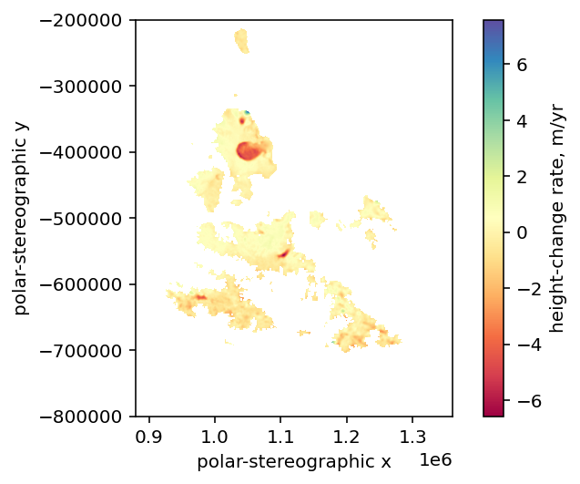
The datasets here represent surface-height differences relative to 2020.0. For a quick view of what is going on, we can make a map of the mean height change rate from the start of the mission to the present:
# note that time is in days after Jan 1 2018dhdt=(ds['delta_h'][-1,:,:]-ds['delta_h'][0,:,:])/(ds['time'][-1]-ds['time'][0])*365.25extent=np.array([np.min(ds['x'])-500,np.max(ds['x'])+500,np.min(ds['y'])-500,np.max(ds['y'])+500])
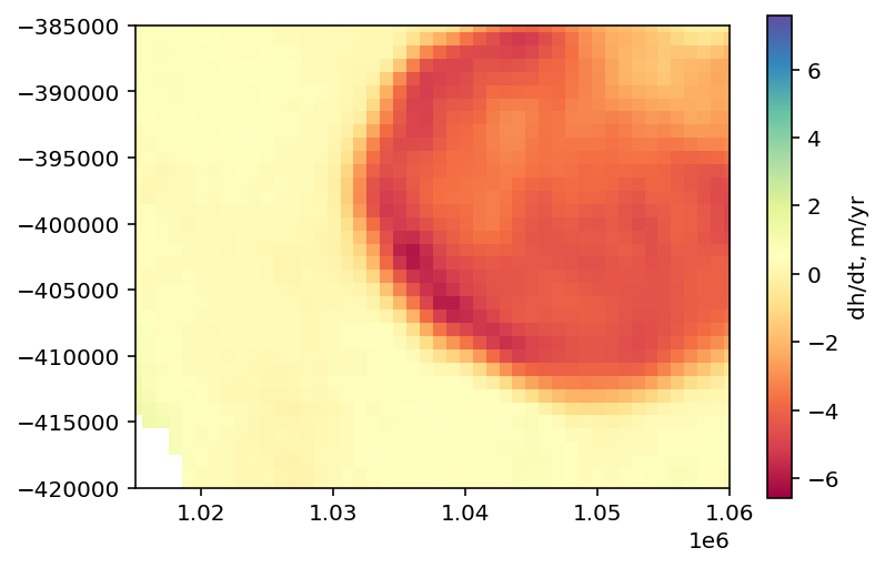
If you are looking at the map in interactive mode (%matplotlib widget in the first cell) you can use the box-zoom button to zoom in on the edge of the surging glacier, or you can run the next cell to zoom to pre-selected region:
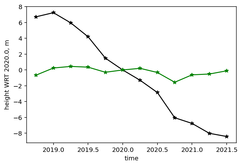
If we want to see the height change for a point, we can find the x and y coordinates that are closest to that point, and plot the delta_h variable for those coordinates. Let’s do that for the point a the center of the current zoomed view, and for another point 12 km to the left:
# get the limits of the current axes, mark the centerXR=np.array(ax1.get_xlim())#<----------In interactive mode, try zooming in on a different locationYR=np.array(ax1.get_ylim())xc=XR.mean()yc=YR.mean()# find the point closest to the axes center:col=np.argmin(np.abs(np.array(ds.x)-xc))row=np.argmin(np.abs(np.array(ds.y)-yc))ax1.plot(ds.x[col],ds.y[row],'k*')plt.figure()ax2=plt.gca()ax2.plot(ds.time/365.25+2018,ds.delta_h[:,row,col],'k',marker='*')# find another point 12 km to the left of the center:col=np.argmin(np.abs(np.array(ds.x)-(xc-12000)))row=np.argmin(np.abs(np.array(ds.y)-yc))ax1.plot(ds.x[col],ds.y[row],'g*')ax2.plot(ds.time/365.25+2018,ds.delta_h[:,row,col],'g',marker='*')ax2.set_xlabel('time');ax2.set_ylabel('height WRT 2020.0, m');
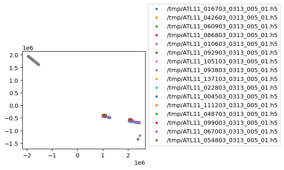
We might be interested to see where these height changes come from. ATL15 is derived from the ATL11 (along-track height change) product, which maps height changes for individual ICESat-2 reference tracks. We don’t necessarily know what track has contributed to the height change at any given point, so we need to bring in some more data-discovery tools to get there.
We can use a CMR (Common Metadata Repository) query through icepyx to find what ATL11 granules have contributed to the height changes we see above. CMR queries are conducted in latitude and longitude, rather than projected coordinates, so we’ll need to find the latitude and longitude for the zoomed-in axes using pyproj:
# Prepare coordinate transformations between lat/lon and the ATL15 coordinate systemcrs=CRS.from_epsg(3413)to_xy_crs=Transformer.from_crs(crs.geodetic_crs,crs)to_geo_crs=Transformer.from_crs(crs,crs.geodetic_crs)corners_lat,corners_lon=to_geo_crs.transform(np.array(XR)[[0,1,1,0,0]],np.array(YR)[[0,0,1,1,0]])latlims=[np.min(corners_lat),np.max(corners_lat)]lonlims=[np.min(corners_lon),np.max(corners_lon)]
There are a total of 55 granules that intersect our region. This is too many files to download during a tutorial, although it’s not a huge amount of data. Let’s take a peek at the ATL11 filenames to help decide what to download. These filenames follow a specific format:
ATL11_054803_0311_004_01.h5
This name is made up of :
ATL11_ttttrr_c0c1_RRR_VV.h5
where
ATL11 is the product name
tttt is the reference ground track (0548)
rr is the subregion (03 indicates as ascending track in the northern mid latitudes)
c0c1 are the first and last repeat-track cycles in the granule
RRR is the release
VV is the version
The subregion is particularly useful here: region 03 are upper-northern-hemisphere ascending tracks, and region 04 are mid-northern-hemisphere descending tracks. Region 04 crosses the pole. Let’s start by just downloading region 03. We’ll use the shell program ‘wget’ to do the downloads, and a regular expression to capture the region number.
ATL11_re=re.compile('ATL11_(\d\d\d\d)(\d\d)_')forgranuleinregion_a.granules.avail:this_name=granule['producer_granule_id']# check if each granule has been downloaded alreadyifos.path.isfile('/tmp/'+this_name):continue# pull out the subregion number, skip subregion 4subregion=ATL11_re.search(this_name).group(2)ifnotsubregion=='03':continueprint(this_name)! wget {granule['links'][0]['href']} -q -O /tmp/{this_name}
ATL11_004503_0313_005_01.h5
ATL11_010603_0313_005_01.h5
ATL11_016703_0313_005_01.h5
ATL11_022803_0313_005_01.h5
ATL11_042603_0313_005_01.h5
ATL11_048703_0313_005_01.h5
ATL11_054803_0313_005_01.h5
ATL11_060903_0313_005_01.h5
ATL11_067003_0313_005_01.h5
ATL11_086803_0313_005_01.h5
ATL11_092903_0313_005_01.h5
ATL11_093803_0313_005_01.h5
ATL11_099003_0313_005_01.h5
ATL11_105103_0313_005_01.h5
ATL11_111203_0313_005_01.h5
ATL11_137103_0313_005_01.h5
Let’s see what these files look like. An easy way to see what is in these granules is to use the ‘h5ls’ utility:
# look at the last granule downloaded:print(this_name)! h5ls /tmp/{this_name}
ATL11_137103_0313_005_01.h5
METADATA                 Group
ancillary_data           Group
orbit_info               Group
pt1                      Group
pt2                      Group
pt3                      Group
quality_assessment       Group
The ‘pt1’,’pt2’, and ‘pt3’ groups contain data for the left, middle and right pair tracks. It’s in these tracks that we find the data:
! h5ls /tmp/{this_name}/pt2
crossing_track_data      Group
cycle_number             Dataset {11}
cycle_stats              Group
delta_time               Dataset {1473, 11}
h_corr                   Dataset {1473, 11}
h_corr_sigma             Dataset {1473, 11}
h_corr_sigma_systematic  Dataset {1473, 11}
latitude                 Dataset {1473}
longitude                Dataset {1473}
quality_summary          Dataset {1473, 11}
ref_pt                   Dataset {1473}
ref_surf                 Group
Here we see ‘latitude’, ‘longitude’, ‘delta_time’, and ‘h_corr’, which give the location, timing, and height of the data.
To look at the data in the ATL11 files, we will use the h5py package. We’ll
Store the data from each file in a dictionary
Store the file-level data in another dictionary
file_xyth={}# use the glob package to find the ATL11s that we downloadedforfileinglob.glob('/tmp/ATL11*.h5'):withh5py.File(file,'r')ash5f:try:lat=np.array(h5f['pt2']['latitude'])lon=np.array(h5f['pt2']['longitude'])exceptException:passx,y=to_xy_crs.transform(lat,lon)file_xyth[file]={'x':x,'y':y,'h':np.array(h5f['pt2']['h_corr']),'t':np.array(h5f['pt2']['delta_time'])}# read the height valuestemp=np.array(h5f['pt2']['h_corr'])# identify invalid heights, and set them to NaNtemp[temp==h5f['pt2/']['h_corr'].attrs['_FillValue']]=np.NaN# store the data in a second dictionary:file_xyth[file]['h']=temp
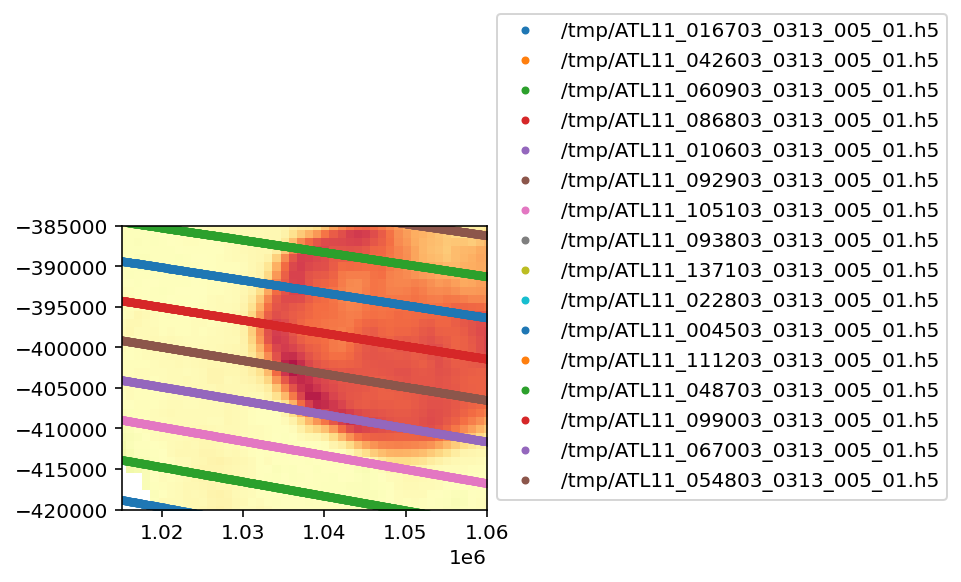
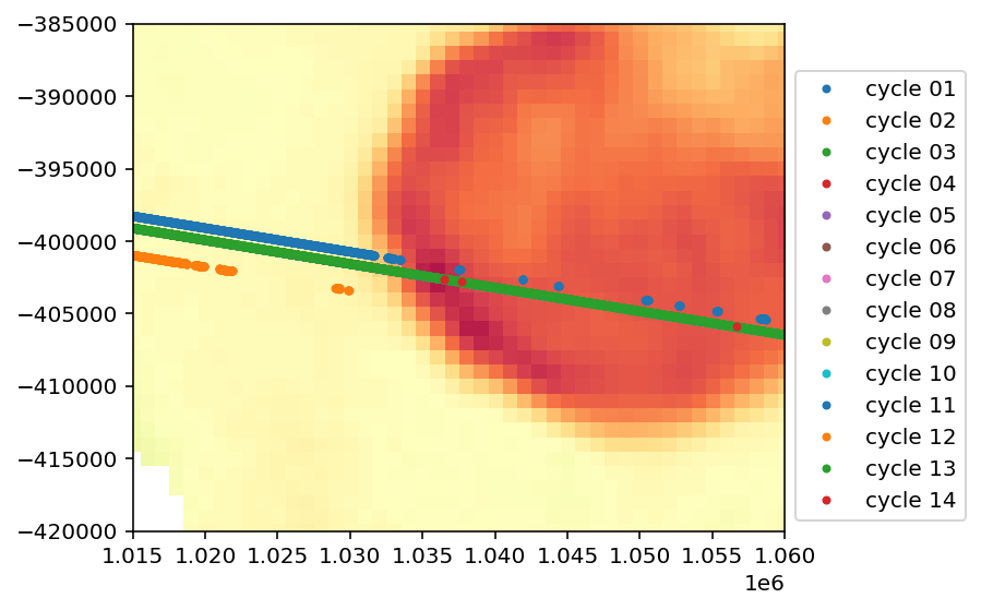
The granules extend well beyond our region of interest, but if you zoom in on the edge of the surge region, you’ll see that they all hit (or come close to hitting) the region we specified.
# zoomed-in version for rendered tutorial:plt.figure();plt.imshow(dhdt,cmap='Spectral',extent=extent)plt.gca().set_aspect(1)forfilename,Dinfile_xyth.items():plt.plot(D['x'],D['y'],'.',label=filename)plt.gca().set_xlim(XR)plt.gca().set_ylim(YR)plt.legend(loc='lower left',bbox_to_anchor=[1,0])plt.tight_layout()
Let’s find the points that are within our bounding box for one of the files (the pink one in the plot we just made). We’ll use the glob package to find an example on track 548
ATL11_file=glob.glob('/tmp/ATL11_0548*')[0]print(f"ATL11 file is {ATL11_file}")xyth=file_xyth[ATL11_file]#<---------- Try a different ATL11 file here!ind=xyth['x']>XR[0]ind&=xyth['x']<XR[1]ind&=xyth['y']>YR[0]ind&=xyth['y']<YR[1]
ATL11 file is /tmp/ATL11_054803_0313_005_01.h5
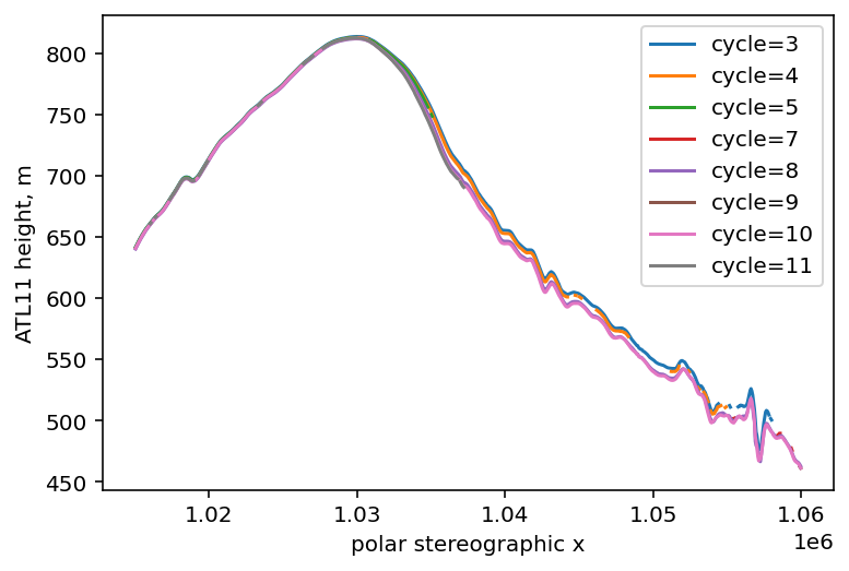
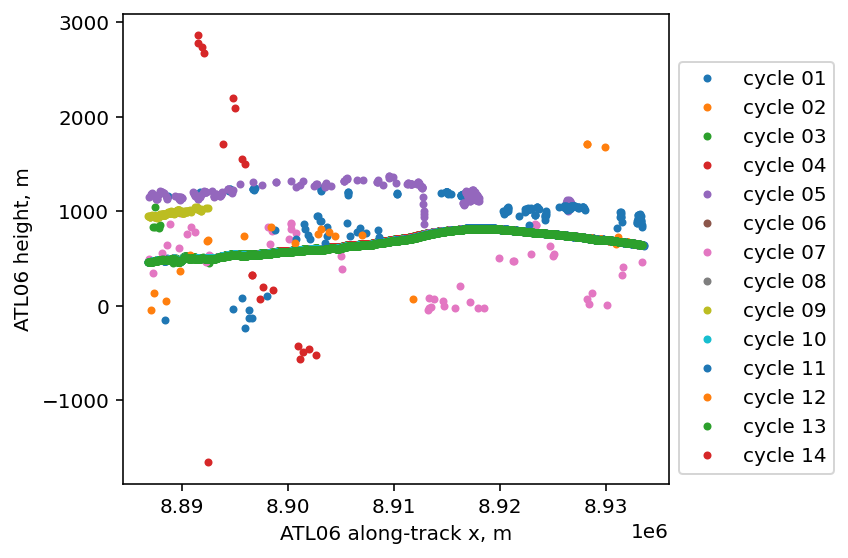
To get an idea of what’s in the file, we’ll plot the heights against the projected x coordinate for the data.
plt.figure();forcycleinrange(3,12):# Cycles in the ATL11 run from 3 to 11, so each cycle's data is in the cycle-3rd columnifnp.any(np.isfinite(xyth['h'][ind,cycle-3])):plt.plot(xyth['x'][ind],xyth['h'][ind,cycle-3],label=f'cycle={cycle}')plt.legend()plt.gca().set_xlabel('polar stereographic x')plt.gca().set_ylabel('ATL11 height, m');
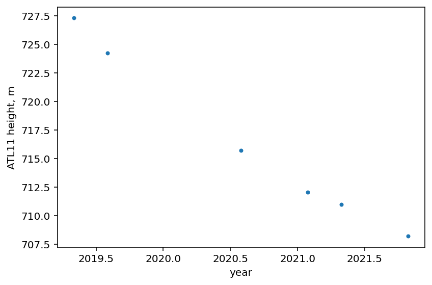
We can see that on the left-hand side of the ice cap, the height has been constant in time, but the right-hand side of the track samples the region that is thinning rapidly. Let’s find the data for a point in the thinning region and plot it:
# find the data close to x=1.036e6 ind_11=np.argmin(np.abs(xyth['x']-1.036e6))#<-------------Try a different x location hereplt.figure()plt.plot(xyth['t'][ind_11,:]/24/3600/365.25+2018,xyth['h'][ind_11,:],'.')plt.gca().set_ylabel('ATL11 height, m')plt.gca().set_xlabel('year')plt.tight_layout()
ATL11 data are generated by combining ALT06 data collected over the same ground track, for different cycles. We can use CMR to identify data from a specific ground track, and we can look at our ATL11 filenames to see what
Next, let’s look at the ATL06 data that were used to generate the ATL11 data. If we can acquire the ATL06 files for RGT 0548, subregion 03, we’ll have the data that went into this ATL11.
Let’s try icePyx to query CMR again to look for these data. We can use the same query as before, but requesting ATL06, and specifying the ‘tracks’ keyword to obtain only RGT 0548. Our search box is right on a region boundary, so we’ll check the filenames to obtain only region 3.
{'Number of available granules': 28,
 'Average size of granules (MB)': 5.203098433364285,
 'Total size of all granules (MB)': 145.68675613419995}
As before, we can download these granules using wget, using a regular expression to check that each file is actually in our region:
# this regular expression matches the track number, the cycle, and the region # in an ATL06 filenameATL06_re=re.compile('ATL06_\d+_(\d\d\d\d)(\d\d)(\d\d)_')forgranuleinregion_b.granules.avail:this_name=granule['producer_granule_id']# skip the granule if we're not in region 03ifnotATL06_re.search(this_name).group(3)=="03":continue# check if each granule has been downloaded alreadyifos.path.isfile('/tmp/'+this_name):continueprint(this_name)! wget -nc {granule['links'][0]['href']} -q -O /tmp/{this_name}
And, as before, we can look at the contents of one of these granules using h5ls. As before, we’ll use glob to select the rgt and cycle we want:
# pick cycle 5 on track 548ATL06_file=glob.glob('/tmp/ATL06*_054805*.h5')[0]print(f"ATL06 file is {ATL06_file}")! h5ls {ATL06_file}
ATL06 file is /tmp/ATL06_20191101185115_05480503_005_01.h5
METADATA                 Group
ancillary_data           Group
gt1l                     Group
gt1r                     Group
gt2l                     Group
gt2r                     Group
gt3l                     Group
gt3r                     Group
orbit_info               Group
quality_assessment       Group
The latitude, longitude, and height data are in the gtxx/land_ice_segments group:
! h5ls {ATL06_file}/gt2l/land_ice_segments
atl06_quality_summary    Dataset {3484/Inf}
bias_correction          Group
delta_time               Dataset {3484/Inf}
dem                      Group
fit_statistics           Group
geophysical              Group
ground_track             Group
h_li                     Dataset {3484/Inf}
h_li_sigma               Dataset {3484/Inf}
latitude                 Dataset {3484/Inf}
longitude                Dataset {3484/Inf}
segment_id               Dataset {3484/Inf}
sigma_geo_h              Dataset {3484/Inf}
Let’s read the data, and store them in a dictionary. We’ll also parse the filename to get the cycle for each file.
cycle_D6={}forfileinsorted(glob.glob('/tmp/ATL06*.h5')):this_D={}withh5py.File(file,'r')ash5f:forfieldin['latitude','longitude','h_li','atl06_quality_summary','ground_track/x_atc']:temp=np.array(h5f['gt2r/land_ice_segments'][field])try:temp[temp==h5f['gt2r/land_ice_segments'][field].attrs['_FillValue']]=np.NaNexceptKeyError:pass# handle the 'ground_track/x_atc' fieldif'/'infield:field=field.split('/')[1]this_D[field]=tempthis_D['x'],this_D['y']=to_xy_crs.transform(this_D['latitude'],this_D['longitude'])cycle_D6[ATL06_re.search(file).group(2)]=this_D
Let’s also figure out what points are within our region of interest:
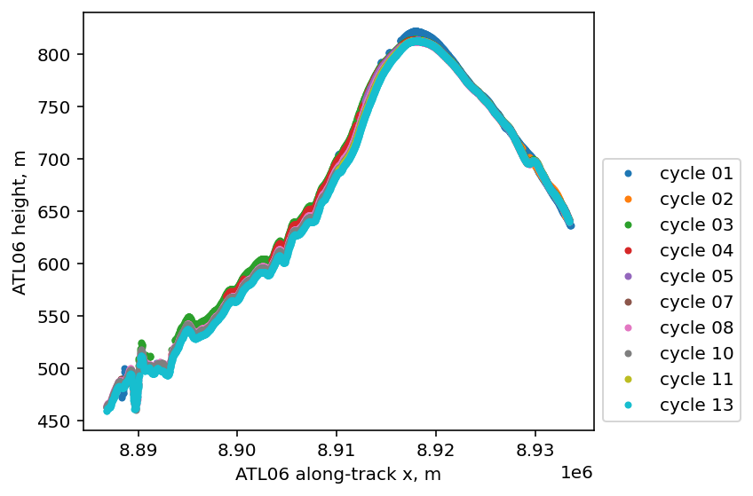
This doesn’t look promising. We have lots of height values that look nothing like a glacier, much less an island. Fortunately, ATL06 comes with a quality flag (atl06_quality_summary) that identifies segments that are likely good (zero means no problems).
Now we can see what we wanted to see. The data now run from south to north (the opposite orientation from the previous plots), but we can see where the height is changing. The height-change signal is somewhat obscured because the tracks are not exactly on top of one another, unlike in ATL11, where the across-track slope is taken into account.
To go one level deeper, we’ll move to a different tool. The SlideRule project provides ATL03 photon data from a convenient web API. We’ll request data for one cycle, and show the photon heights and classifications. SlideRule can query specific ATL03 files, and we can determine what ATL03 we want based on the ATL06 filenames we already have. (SlideRule can also do CMR queries, but for the purposes of this tutorial, it’s easiest to choose a specific file).
The SlideRule atl03s function returns a pandas dataFrame containing photon-level data:
temp[0:5]
track
segment_id
segment_dist
cycle
rgt
sc_orient
quality_ph
delta_time
yapc_score
atl03_cnf
distance
height
atl08_class
pair
geometry
time
2019-08-02 23:16:39.241362264
2
443606
8.889489e+06
4
548
0
0
5.002300e+07
0
0
-5.029457
874.687378
4
0
POINT (23.98961 79.57145)
2019-08-02 23:16:39.241362264
2
443606
8.889489e+06
4
548
0
0
5.002300e+07
0
0
-4.364876
744.842407
4
0
POINT (23.98961 79.57145)
2019-08-02 23:16:39.241362264
2
443606
8.889489e+06
4
548
0
0
5.002300e+07
0
0
-4.281098
728.471130
4
0
POINT (23.98961 79.57145)
2019-08-02 23:16:39.241362264
2
443606
8.889489e+06
4
548
0
0
5.002300e+07
0
0
-3.417146
559.688721
4
0
POINT (23.98961 79.57146)
2019-08-02 23:16:39.241362264
2
443606
8.889489e+06
4
548
0
0
5.002300e+07
0
0
-3.510730
577.963257
4
0
POINT (23.98961 79.57146)
In SlideRule, the nomenclature is a little different from elsewhere in the ICESat-2 project : a ‘track’ in SlideRule is a ‘Pair’ elsewhere, and the ‘pair’ variable distinguishes the left and right beams in an ICESat-2 beam pair.
5.1 Plotting ATL03 photon heights and confidence values:
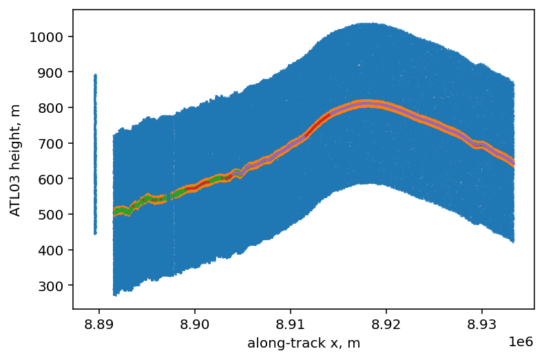
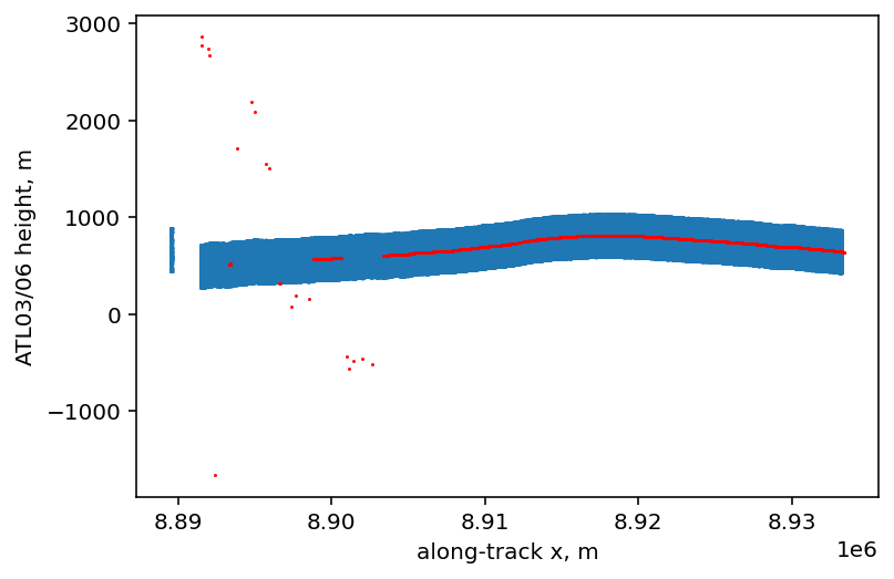
To plot the data, we’ll obtain the along-track location information using the ‘segment_dist’ and ‘distance’ fields in the dataframe, and use the ‘atl03_cnf’ (confidence that the photon is not noise) to color-code each photon:
temp_p=temp[temp.pair==0]D6=cycle_D6['04']# get the ATL06 data from cycle 4plt.figure();colors=['black','gray','blue','red','orange']forq_val,colorinzip(np.arange(5),colors):these=temp_p['atl03_cnf']==q_valplt.plot(temp_p['segment_dist'][these]+temp_p['distance'][these],temp_p.height[these],'.',markersize=0.5)plt.gca().set_xlabel('along-track x, m')plt.gca().set_ylabel('ATL03 height, m')
Text(0, 0.5, 'ATL03 height, m')
We can also overlay the ATL06 segment heights on the plot:
Thanks for following along. If you look back through the code above, there are a few different places where you can change the regions and the tracks, and see how different data look. Later on in the hack week you’ll see different (better) ways to do some of the tasks that we’ve done here, but the basic tools (h5py, h5ls, and numpy) are good to have on hand to help debug some of the more advanced techniques. Happy hacking!